Around the numeric-symbolic
computation
of differential Galois
groups |
|
|
Dépt. de
Mathématiques
(bât. 425)
Université Paris-Sud
91405 Orsay Cedex
France
|
|
Email:
vdhoeven@texmacs.org
|
|
|
|
Let  be a linear differential
operator, where be a linear differential
operator, where  is an effective
algebraically closed subfield of is an effective
algebraically closed subfield of  . It
can be shown that the differential Galois group of . It
can be shown that the differential Galois group of  is generated (as a closed algebraic group) by
a finite number of monodromy matrices, Stokes matrices and
matrices in local exponential groups. Moreover, there exist
fast algorithms for the approximation of the entries of
these matrices. is generated (as a closed algebraic group) by
a finite number of monodromy matrices, Stokes matrices and
matrices in local exponential groups. Moreover, there exist
fast algorithms for the approximation of the entries of
these matrices.
In this paper, we present a numeric-symbolic algorithm for
the computation of the closed algebraic subgroup generated
by a finite number of invertible matrices. Using the above
results, this yields an algorithm for the computation of
differential Galois groups, when computing with a sufficient
precision.
Even though there is no straightforward way to find a
“sufficient precision” for guaranteeing the
correctness of the end-result, it is often possible to check
a posteriori whether the end-result is correct. In
particular, we present a non-heuristic algorithm for the
factorization of linear differential operators.
|

1.Introduction
Let be a monic linear differential operator of
order  , where is an
effective algebraically closed subfield of . A
holonomic function is a solution to the equation
, where is an
effective algebraically closed subfield of . A
holonomic function is a solution to the equation  .
The differential Galois group
.
The differential Galois group  of is a linear algebraic group which acts on the space
  of solutions (see section 2.2 and [Kap57, vdPS03, Kol73]). It carries a
lot of information about the solutions in and on
the relations between different solutions. For instance, the existence
of non-trivial factorizations of and the
existence of Liouvillian solutions can be read off from the Galois
group. This makes it an interesting problem to explicitly compute the
Galois group of .
of solutions (see section 2.2 and [Kap57, vdPS03, Kol73]). It carries a
lot of information about the solutions in and on
the relations between different solutions. For instance, the existence
of non-trivial factorizations of and the
existence of Liouvillian solutions can be read off from the Galois
group. This makes it an interesting problem to explicitly compute the
Galois group of .
A classical approach in this area is to let act
on other vector spaces obtained from by the
constructions from linear algebra, such as symmetric powers  and exterior powers
  [Bek94,
SU93]. For a suitable such space
[Bek94,
SU93]. For a suitable such space  ,
the Galois group consists precisely of those
invertible
,
the Galois group consists precisely of those
invertible  matrices which leave a certain
one-dimensional subspace of invariant [Hum81,
chapter 11]. Invariants in or
under may be computed more efficiently by
considering the local solutions of at
singularities [vHW97, vH97, vH96].
More recently, and assuming (for instance) that the coefficients of are actually in
matrices which leave a certain
one-dimensional subspace of invariant [Hum81,
chapter 11]. Invariants in or
under may be computed more efficiently by
considering the local solutions of at
singularities [vHW97, vH97, vH96].
More recently, and assuming (for instance) that the coefficients of are actually in  , alternative
algorithms appeared which are based on the reduction of the equation
modulo a prime number
, alternative
algorithms appeared which are based on the reduction of the equation
modulo a prime number  [Clu04, vdP95, vdPS03].
In this paper, we will study another type of “analytic
modular” algorithms, by studying the operator
in greater detail near its singularities using the theory of
accelero-summation [É85, É87, É92, É93, Bra91, Bra92]. More precisely, we will use the following facts:
-
The differential Galois group of is generated
(as a closed algebraic group) by a finite number of monodromy
matrices, Stokes matrices and matrices in so called local exponential
groups.
-
There exists an algorithm [vdH99, vdH01b, vdH05b] for the approximation of the entries of the above
matrices. If
 is the algebraic closure of
  , then
  -digit approximations
can be computed in time
-digit approximations
can be computed in time  .
.
When using these facts for the computation of differential Galois
groups, the bulk of the computations is reduced to linear algebra in
dimension with multiple precision coefficients.
In comparison with previous methods, this approach is expected to be
much faster than algorithms which rely on the use of exterior powers. A
detailed comparison with arithmetic modular methods would be
interesting. One advantage of arithmetic methods is that they are easier
to implement in existing systems. On the other hand, our analytic
approach relies on linear algebra in dimension
(with floating coefficients), whereas modulo
methods rely on linear algebra in dimension  (with coefficients modulo ), so the first
approach might be a bit faster. Another advantage of the analytic
approach is that it is more easily adapted to coefficients fields with transcendental constants.
(with coefficients modulo ), so the first
approach might be a bit faster. Another advantage of the analytic
approach is that it is more easily adapted to coefficients fields with transcendental constants.
Let us outline the structure of this paper. In section 2,
we start by recalling some standard terminology and we shortly review
the theorems on which our algorithms rely. We start with a survey of
differential Galois theory, monodromy and local exponential groups. We
next recall some basic definitions and theorems from the theory of
accelero-summation and the link with Stokes matrices and differential
Galois groups. We finally recall some theorems about the effective
approximation of the transcendental numbers involved in the whole
process.
Before coming to the computation of differential Galois groups, we first
consider the simpler problem of factoring in
section 3. We recall that there exists a non-trivial
factorization of if and only if the Galois group
of admits a non-trivial invariant subspace. By
using computations with limited precision, we show how to use this
criterion in order to compute candidate factorizations or a proof that
there exist no factorizations. It is easy to check a posteriori
whether a candidate factorization is correct, so we obtain a
factorization algorithm by increasing the precision until we obtain a
correct candidate or a proof that there are no factorizations.
In section 4 we consider the problem of computing the
differential Galois group of . Using the results
from section 2, it suffices to show how to compute the
algebraic closure of a matrix group generated by
a finite number of given elements. A theoretical solution for this
problem based on Gröbner basis techniques has been given in [DJK03]. The main idea behind the present algorithm is similar,
but more emphasis is put on efficiency (in contrast to generality).
First of all, in our context of complex numbers with arbitrary
precisions, we may use the LLL-algorithm for the computation of linear
and multiplicative dependencies [LLL82]. Secondly, the
connected component of is represented as the
exponential of a Lie algebra  given by a basis.
Computations with such Lie algebras essentially boil down to linear
algebra. Finally, we use classical techniques for finite groups in order
to represent and compute with the elements in
given by a basis.
Computations with such Lie algebras essentially boil down to linear
algebra. Finally, we use classical techniques for finite groups in order
to represent and compute with the elements in  [Sim70, Sim71, MO95]. Moreover,
we will present an algorithm for non-commutative lattice reduction,
similar to the LLL-algorithm, for the efficient computation with
elements in near the identity.
[Sim70, Sim71, MO95]. Moreover,
we will present an algorithm for non-commutative lattice reduction,
similar to the LLL-algorithm, for the efficient computation with
elements in near the identity.
The algorithms in section 4 are all done using a fixed
precision. Although we do prove that we really compute the Galois group
when using a sufficiently large precision, it is not clear a
priori how to find such a “sufficient precision”.
Nevertheless, we have already seen in section 3 that it is
often possible to check the correctness of the result a
posteriori, especially when we are not interested in the Galois
group itself, but only in some information
provided by . Also, it might be possible to
reduce the amount of dependence on “transcendental
arguments” in the algorithm modulo a further development of our
ideas. Some hints are given in the last section.
Remark 1. The author first suggested the main
approach behind this paper during his visit at the MSRI in 1998. The
outline of the algorithm in section 4.5 came up in a
discussion with Harm Derksen (see also [DJK03]). The little
interest manifested by specialists in effective differential Galois
theory for this approach is probably due to the fact that current
computer algebra systems have very poor support for analytic
computations. We hope that the present article will convince people to
put more effort in the implementation of such algorithms. We started
such an effort [vdHea05], but any help would be
appreciated. Currently, none of the algorithms presented in this paper
has been implemented.
2.Preliminaries
2.1.Notations
Throughout this paper, we will use the following notations:
-

-
An algebraically closed field of constants.
-

-
The algebra of matrices with coefficients in
.
-

-
The subgroup of of invertible matrices.
-

-
The vector space generated by a subset of a
larger vector space.
-

-
The algebra generated by a subset of a larger
algebra.
Vectors are typeset in bold face  and we use the
following vector notations:
and we use the
following vector notations:

Matrices  will also be used as mappings
  . When making a base change in
  , we
understand that we perform the corresponding transformations
, we
understand that we perform the corresponding transformations  on all matrices under consideration. We denote
  for the diagonal matrix with entries
  .
The
.
The  may either be scalars or square matrices.
Given a matrix and a vector
may either be scalars or square matrices.
Given a matrix and a vector  ,
we write
,
we write  for the vector
  with
with  for all
  .
.
2.2.Differential Galois
groups
Consider a monic linear differential operator  ,
where is an algebraically closed subfield of
and
,
where is an algebraically closed subfield of
and  . We will denote by
 the finite set of singularities of (in the case of
  , one considers the
transformation
, one considers the
transformation  ). A Picard-Vessiot
extension of
). A Picard-Vessiot
extension of  is a differential field
  such that
-
PV1
-
 is differentially generated by and a basis of solutions
  to the
equation .
to the
equation .
-
PV2
-
 has as its field of
constants.
has as its field of
constants.
A Picard-Vessiot extension always exists: given a point  and
and  , let
, let  be the unique
solution to with
be the unique
solution to with  for
for
 . We call
  the
canonical basis for the solution space of
at
the
canonical basis for the solution space of
at  , and regard
  as a
column vector. Taking , the condition
PV2 is trivially satisfied since
as a
column vector. Taking , the condition
PV2 is trivially satisfied since  and the constant field of
  is .
is .
Let be a Picard-Vessiot extension of and let  be as in
PV1. The differential Galois group
be as in
PV1. The differential Galois group  of the extension
  is the group of
differential automorphisms which leave pointwise
invariant. It is classical [Kol73] that
is independent (up to isomorphism) of the particular choice of the
Picard-Vessiot extension .
is the group of
differential automorphisms which leave pointwise
invariant. It is classical [Kol73] that
is independent (up to isomorphism) of the particular choice of the
Picard-Vessiot extension .
Given an automorphism  , any solution
  to is sent to another solution. In
particular, there exists a unique matrix
to is sent to another solution. In
particular, there exists a unique matrix  with
with
 for all . This yields an
embedding
for all . This yields an
embedding  of into and we define
  . Conversely,
 belongs to
  if every
differential relation
if every
differential relation  satisfied by
  is also satisfied by
  (with
(with  ). Since this assumption constitutes an infinite
number of algebraic conditions on the coefficients of
). Since this assumption constitutes an infinite
number of algebraic conditions on the coefficients of  ,
it follows that is a Zariski closed algebraic
matrix group. Whenever
,
it follows that is a Zariski closed algebraic
matrix group. Whenever  is another basis, we
obtain the same matrix group
is another basis, we
obtain the same matrix group  up to conjugation.
Assume now that  is a larger algebraically closed
subfield of . Then the field
is a larger algebraically closed
subfield of . Then the field  is again a Picard-Vessiot extension of
  .
Furthermore, the Ritt-Raudenbush theorem [Rit50] implies
that the perfect differential ideal of all with
is finitely generated, say by
.
Furthermore, the Ritt-Raudenbush theorem [Rit50] implies
that the perfect differential ideal of all with
is finitely generated, say by  .
But then is still a finite system of generators
of the perfect differential ideal of all
.
But then is still a finite system of generators
of the perfect differential ideal of all  with
. Consequently,
with
. Consequently,  (i.e. as an algebraic group over
  )
is determined by the same algebraic equations as
)
is determined by the same algebraic equations as  .
We conclude that
.
We conclude that  .
.
Let be a Picard-Vessiot extension of . Any differential field with  naturally induces an algebraic subgroup
  of automorphisms of which leave
fixed. Inversely, any algebraic subgroup
of automorphisms of which leave
fixed. Inversely, any algebraic subgroup  of
of  gives rise to the
differential field
gives rise to the
differential field  with
with  of all elements which are invariant under the action of .
We say that (resp. )
is closed if
of all elements which are invariant under the action of .
We say that (resp. )
is closed if  (resp.
  ). In that case, the extension
  is said to be normal, i.e. every element in
  is moved by an automorphism of
over . The main theorem from differential Galois
theory states that the Galois correspondences are bijective [Kap57,
Theorem 5.9].
is moved by an automorphism of
over . The main theorem from differential Galois
theory states that the Galois correspondences are bijective [Kap57,
Theorem 5.9].
Theorem 2. With the above notations:
-
The correspondences
 and
and  are bijective.
-
The group is a closed normal subgroup of
if and only if the extension
 is normal. In that case,
  .
.
Corollary 3. Let  .
If
.
If  for all
  , then
  .
.
2.3.Monodromy
Consider a continuous path  on
on  from
from  to
to  . Then analytic
continuation of the canonical basis
. Then analytic
continuation of the canonical basis  at along yields a basis of solutions
to at
at along yields a basis of solutions
to at  . The matrix
  with
with
 |
(1) |
is called the connection matrix or transition matrix
along . In particular, if  ,
then we call
,
then we call  a monodromy matrix based
in . We clearly have
a monodromy matrix based
in . We clearly have
for the composition of paths, so the monodromy matrices based in form a group  which is called
the monodromy group. Given a path from
to , we notice that
which is called
the monodromy group. Given a path from
to , we notice that  . Since any differential relation satisfied by is again satisfied by its analytic continuation along
, we have
. Since any differential relation satisfied by is again satisfied by its analytic continuation along
, we have  and
and  .
.
Remark 4. The definition of transition matrices
can be slightly changed depending on the purpose [vdH05b,
Section 4.3.1]: when interpreting and  as row vectors, then (1) has to be
transposed. The roles of and
may also be interchanged modulo inversion of .
as row vectors, then (1) has to be
transposed. The roles of and
may also be interchanged modulo inversion of .
Now assume that admits a singularity at  (if
(if  then we may reduce to
this case modulo a translation; singularities at infinity may be brought
back to zero using the transformation
then we may reduce to
this case modulo a translation; singularities at infinity may be brought
back to zero using the transformation  ). It is
well-known [Fab85, vH96] that
). It is
well-known [Fab85, vH96] that  admits a computable formal basis of solutions of the form
 |
(2) |
with  ,
,  ,
,  and
and  . We will denote by
  the set of finite sums of expressions of the form (2). We
may see as a differential subring of a formal
differential field of “complex transseries”
the set of finite sums of expressions of the form (2). We
may see as a differential subring of a formal
differential field of “complex transseries”  [vdH01a] with constant field .
We recall that transseries in are infinite
linear combinations  of
“transmonomials” with “grid-based support”. The
set
of
“transmonomials” with “grid-based support”. The
set  of transmonomials forms a totally ordered
vector space for exponentiation by reals and the asymptotic ordering
of transmonomials forms a totally ordered
vector space for exponentiation by reals and the asymptotic ordering
 . In particular, each non-zero transseries admits a unique dominant monomial
  .
It can be shown [vdH01a] that there exists a unique basis
.
It can be shown [vdH01a] that there exists a unique basis
 of solutions to of the
form (2), with
of solutions to of the
form (2), with  and
and  for all
  . We call
  the
canonical basis of solutions in and there is an
algorithm which computes as a function of .
the
canonical basis of solutions in and there is an
algorithm which computes as a function of .
Let  be the subset of of
all finite sums of expressions of the form (2) with
be the subset of of
all finite sums of expressions of the form (2) with  . Then any
  can uniquely be
written as a finite sum
can uniquely be
written as a finite sum  , where
  .
Let
.
Let  be the group of all automorphisms
  for which there exists a mapping
  with
with  for all . Then every
 preserves differentiation and maps the
Picard-Vessiot extension of
into itself. In particular, the restriction
preserves differentiation and maps the
Picard-Vessiot extension of
into itself. In particular, the restriction  of
to is a subset of .
of
to is a subset of .
Proposition 5. Assume that  is fixed under
  . Then
  .
.
Proof. Assume that

and
let

be an exponential with

.
Let

be a supplement of the

-vector
space

. Let

be the
mapping in
which sends

to

for each

and

. Then we clearly have

.
Let  be the set of exponents corresponding to the
exponents of the elements of the canonical basis
be the set of exponents corresponding to the
exponents of the elements of the canonical basis  .
Using linear algebra, we may compute a multiplicatively independent set
.
Using linear algebra, we may compute a multiplicatively independent set
 such that
  for certain
 and all .
Proposition 6. With the above
notations, the algebraic group  is generated by
the matrices
is generated by
the matrices  where
where  is
chosen arbitrarily.
is
chosen arbitrarily.
Proof. Let  be the group
generated by the matrices . Notice that each
individual matrix generates
be the group
generated by the matrices . Notice that each
individual matrix generates  :
assuming
:
assuming  , the variety
  is irreducible of dimension
  and is not contained in an algebraic group of dimension
  . Now any
  is a diagonal
matrix
is a diagonal
matrix  for some multiplicative mapping
  . Hence

Conversely, each element

determines a multiplicative mapping

which
may be further extended to

using Zorn's
lemma and the fact that

is algebraically
closed. It follows that
.
Assume that  and let
  be
the transformation which sends
be
the transformation which sends  to
to  ,
,  to
to  and
and
 to
to  . Then
  preserves differentiation, so any solution to of the form (2) is sent to another solution
of the same form. In particular, there exists a matrix
preserves differentiation, so any solution to of the form (2) is sent to another solution
of the same form. In particular, there exists a matrix  with
with  , called the formal monodromy
matrix around . We have
, called the formal monodromy
matrix around . We have  .
.
Proposition 7. Assume that is fixed under and  . Then
  .
.
Proof. We already know that .
Interpreting  as a polynomial in
  with
with  , we must have
  since
since

Consequently,  is of the form
  and
and
We conclude that

for every

with

, whence

.
2.4.The process of
accelero-summation
Let  be the differential -algebra
of infinitesimal Puiseux series in
be the differential -algebra
of infinitesimal Puiseux series in  for
for  and consider a formal power series solution
  to
to  . The process of
accelero-summation enables to associate an analytic meaning to
. The process of
accelero-summation enables to associate an analytic meaning to  in a sector near the origin of
the Riemann surface
in a sector near the origin of
the Riemann surface  of
of  ,
even in the case when is divergent.
Schematically speaking, we obtain through a
succession of transformations:
,
even in the case when is divergent.
Schematically speaking, we obtain through a
succession of transformations:
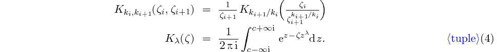
 |
(3) |
Each  is a “resurgent function” which
realizes
is a “resurgent function” which
realizes  in the “convolution model”
with respect to the -th “critical
time”
in the “convolution model”
with respect to the -th “critical
time”  (with
(with  and
and
 ). In our case, is an
analytic function which admits only a finite number of singularities
above . In general, the singularities of a
resurgent function are usually located on a finitely generated grid. Let
us describe the transformations
). In our case, is an
analytic function which admits only a finite number of singularities
above . In general, the singularities of a
resurgent function are usually located on a finitely generated grid. Let
us describe the transformations  ,
,  and
and  in more detail.
The Borel transform
We start by
applying the formal Borel transform to the series  . This transformation sends each
  to
to
where  , and extends by strong linearity:
The result is a formal series  in
in  which converges near the origin of .
The formal Borel transform is a morphism of differential algebras which
sends multiplication to the convolution product, i.e.
which converges near the origin of .
The formal Borel transform is a morphism of differential algebras which
sends multiplication to the convolution product, i.e.  .
.
Accelerations
Given  , the function is defined near the
origin of , can be analytically continued on the
axis
, the function is defined near the
origin of , can be analytically continued on the
axis  , and admits a growth of the form
  at infinity. The next function
  is
obtained from by an acceleration of the
form
is
obtained from by an acceleration of the
form

where the acceleration kernel  is given by
For large  on an axis with
 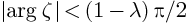 ,
it can be shown that
,
it can be shown that 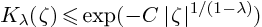 for some constant
  . Assuming that
  satisfies
 |
(5) |
it follows that the acceleration of is well-defined for small  on
on  . The set
  of directions
  such admits a singularity on
 is called the set of Stokes directions.
Accelerations are morphisms of differential -algebras
which preserve the convolution product.
is called the set of Stokes directions.
Accelerations are morphisms of differential -algebras
which preserve the convolution product.
The Laplace transform
The last
function  is defined near the origin of , can be analytically continued on the axis and admits at most exponential growth at infinity. The
function is now obtained using the analytic
Laplace transform
is defined near the origin of , can be analytically continued on the axis and admits at most exponential growth at infinity. The
function is now obtained using the analytic
Laplace transform

On an axis with
 |
(6) |
the function  is defined for all sufficiently
small
is defined for all sufficiently
small  . The set
  of Stokes
directions is defined in a similar way as in the case of accelerations.
The Laplace transform is a morphism of differential -algebras
which is inverse to the Borel transform and sends the convolution
product to multiplication.
of Stokes
directions is defined in a similar way as in the case of accelerations.
The Laplace transform is a morphism of differential -algebras
which is inverse to the Borel transform and sends the convolution
product to multiplication.
Remark 8. Intuitively speaking, one has  .
.
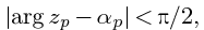
Given critical times in  and directions
  satisfying (5), we
say that a formal power series
satisfying (5), we
say that a formal power series  is
accelero-summable in the multi-direction
is
accelero-summable in the multi-direction  if the above scheme yields an analytic function
  near the origin of any axis on satisfying (6). We denote the set of such power series by
  ,
where
,
where  . Inversely, given
  ,
we denote by
,
we denote by  the set of all triples
  such that
  and so that is well-defined. In that case, we write
  and
and  .
.
The set forms a differential subring of  and the map
  for is injective. If
  and
and  are obtained from
  and
and  by inserting a new critical time and an arbitrary
direction, then we have
by inserting a new critical time and an arbitrary
direction, then we have  . In particular, contains
  , where
  denotes the ring of convergent infinitesimal Puiseux
series. Let
denotes the ring of convergent infinitesimal Puiseux
series. Let  be sets of directions such that each
 is finite modulo
  . Let
. Let
 be the subset of
  of
multi-directions which verify (5).
We denote
of
multi-directions which verify (5).
We denote  ,
,  and
and  .
.
Taking  , the notion of accelero-summation extends
to formal expressions of the form (2) and more general
elements of as follows. Given
, the notion of accelero-summation extends
to formal expressions of the form (2) and more general
elements of as follows. Given  ,
,
 ,
,  and
and  ,
we simply define
,
we simply define  . It can be checked that this
definition is coherent when replacing
. It can be checked that this
definition is coherent when replacing  by
by  for some
  . By linearity, we
thus obtain a natural differential subalgebra
. By linearity, we
thus obtain a natural differential subalgebra  of
accelero-summable transseries with critical times
and in the multi-direction . We also have natural
analogues
of
accelero-summable transseries with critical times
and in the multi-direction . We also have natural
analogues  and
and  of
of  and
and  .
.
The main result we need from the theory of accelero-summation is the
following theorem [É87, Bra91].
Theorem 9. Let
be a formal solution to . Then  .
.
Corollary 10. Let  be the canonical basis of formal solutions to at
the origin. We have
be the canonical basis of formal solutions to at
the origin. We have  .
.
Proof. Holonomy is preserved under
multiplication with elements of

.
Remark 11. We have aimed to keep our survey of the
accelero-summation process as brief as possible. It is more elegant to
develop this theory using resurgent functions and resurgence monomials
[É85, CNP93].
2.5.The Stokes phenomenon
We say that  is stable under Stokes
morphisms is for all
is stable under Stokes
morphisms is for all  , there exists a
  with
with  , and if the same
property is recursively satisfied by
, and if the same
property is recursively satisfied by  . We denote
by
. We denote
by  the differential subring of
  which is stable under Stokes morphisms. The mappings
  will be called Stokes morphisms and we denote by
  the group of all such maps.
Proposition 12. Assume that is fixed under  . Then
  is convergent.
Proof. Assume that one of the
admits a singularity at  and choose
  maximal and
  minimal. Modulo the
removal of unnecessary critical times, we may assume without loss of
generality that
minimal. Modulo the
removal of unnecessary critical times, we may assume without loss of
generality that  . Let
. Let  with
with  be a multi-direction satisfying (5),
such that
be a multi-direction satisfying (5),
such that  for all
  .
Then
.
Then

for all sufficiently small

. Now
is obtained by integration around

along the axis

. By classical properties of
the Laplace integral [
CNP93, Pré I.2], the
function

cannot vanish, since
admits a singularity in
(if
the Laplace integrals corresponding to both directions

coincide, then the Laplace transform can be
analytically continued to a larger sector, which is only possible if
is analytic in a sector which contains both
directions
). We conclude that

, so
is not fixed under
.
Remark 13. Let  be a set of multi-directions satisfying (5), with
  for exactly one , and so that for all
  , we have
either
, we have
either  or
or  and
and  for some small . For every
 , we have

By looking more carefully at the proof of proposition 12,
we observe that it suffices to assume that is
fixed under all Stokes morphisms of the form  ,
instead of all elements in .
,
instead of all elements in .
We say that  are equivalent, if
  for all , where
  is the denominator of
  . We notice that is finite modulo this equivalent relation. We
denote by
. We notice that is finite modulo this equivalent relation. We
denote by  a subset of
with one element in each equivalence class.
a subset of
with one element in each equivalence class.
Let us now come back to our differential equation .
Given  , the map
  induces
an isomorphism between
induces
an isomorphism between  and
and  .
We denote by
.
We denote by  the unique matrix with
  . Given a second
  , the vector
  is again in
  , whence
  by repeating the argument. In particular, the Stokes
morphism
by repeating the argument. In particular, the Stokes
morphism  induces the Stokes matrix
  .
.
We are now in the position that we can construct a finite set  of generators for the Galois group
  in a regular point
  .
.
Algorithm Compute_generators
return 
Theorem 14. With
constructed as above, the differential Galois group
is generated by as a closed algebraic subgroup
of  .
.
Proof. Assume that
is
fixed by each element of
. We have to prove
that
. Given a singularity

,
let

be the “continuation” of
along

(which involves
analytic continuation until

followed by
“decelero-unsummation”). By proposition
7, we
have

. From proposition
12 and
remark
13, we next deduce that
is
convergent. Indeed, since
, its realization

in the convolution model with critical time
is a function in

.
Consequently,
whenever
and

are equivalent. At this point we have
shown that
is meromorphic at
.
But a function which is meromorphic at all points of the Riemann
sphere
is actually a rational function. It
follows that
.
Remark 15. Slightly less effective versions of
theorem 14 are due to Ramis [Ram85, MR91].
Both papers crucially use previous work by Écalle and we followed
a similar approach as in the second paper. In the Fuchsian case,
i.e. in absence of divergence, the result is due to
Schlesinger [Sch95, Sch97].
Remark 16. We have tried to keep our exposition
as short as possible by considering only “directional
Stokes-morphisms”. In fact, Écalle's theory of resurgent
functions gives a more fine-grained control over what happens in the
convolution model by considering the pointed alien
derivatives  for
for  .
Modulo the identification of functions in the formal model, the
convolution models and the geometric model via accelero-summation, the
pointed alien derivatives commute with the usual derivation
.
Modulo the identification of functions in the formal model, the
convolution models and the geometric model via accelero-summation, the
pointed alien derivatives commute with the usual derivation  . Consequently, if is a solution
to
. Consequently, if is a solution
to  , then we also have
  .
In particular, given the canonical basis of solutions
to , there exists a unique matrix
.
In particular, given the canonical basis of solutions
to , there exists a unique matrix  with
with
This equation is called the bridge equation. Since admits only a finite number of singularities and the
alien derivations “translate singularities”, we have  for some
  , so the matrices
are nilpotent. More generally, if
, so the matrices
are nilpotent. More generally, if  are
are  -linearly independent, then
all elements in the algebra generated by
-linearly independent, then
all elements in the algebra generated by  are
nilpotent.
are
nilpotent.
It is easily shown that the Stokes morphisms correspond to the
exponentials  of directional Alien derivations
 . This yields a way to reinterpret the Stokes
matrices in terms of the with
. This yields a way to reinterpret the Stokes
matrices in terms of the with  .
In particular, the preceding discussion implies that the Stokes
matrices are unipotent. The extra flexibility provided by pointwise
over directional alien derivatives admits many applications, such as
the preservation of realness [Men96]. For further
details, see [É85, É87, É92, É93].
.
In particular, the preceding discussion implies that the Stokes
matrices are unipotent. The extra flexibility provided by pointwise
over directional alien derivatives admits many applications, such as
the preservation of realness [Men96]. For further
details, see [É85, É87, É92, É93].
2.6.Effective complex numbers
A complex number is said to be
effective if there exists an approximation algorithm
for which takes  on input
and which returns an
on input
and which returns an  -approximation
  of for which
  .
The time complexity of this approximation algorithm is the time
.
The time complexity of this approximation algorithm is the time
 it takes to compute a
  -approximation
for . It is not hard to show that the set
-approximation
for . It is not hard to show that the set  of effective complex numbers forms a field. However,
given
of effective complex numbers forms a field. However,
given  the question whether
  is undecidable. The following theorems were proved in [CC90,
vdH99, vdH01b].
is undecidable. The following theorems were proved in [CC90,
vdH99, vdH01b].
Theorem 17. Let  ,
,
 ,
,  and
and  .
Given a broken line path
.
Given a broken line path  on
on  ,
we have
,
we have
-
The value
 of the analytic continuation of
at the end-point of
is effective.
of the analytic continuation of
at the end-point of
is effective.
-
There exists an approximation algorithm of time complexity
 for , when not counting
the approximation time of the input data ,
and
for , when not counting
the approximation time of the input data ,
and  .
.
-
There exists an algorithm which computes an approximation
algorithm for as in (b) as a
function of , and
.
Theorem 18. Let
be regular singular in . Let ,
and . Then  is well-defined for all sufficiently small
  on the effective Riemann surface
  of
of  above , and
-
is effective.
-
There exists an approximation algorithm of time complexity for , when not counting
the approximation time of the input data ,
and .
-
There exists an algorithm which computes an approximation
algorithm for as in (b) as a
function of , and
.
In general, the approximation of involves the
existence of certain bounds. In each of the above theorems, the
assertion (c) essentially states that there exists an algorithm
for computing these bounds as a function of the input data. This
property does not merely follow from (a) and (b)
alone.
The following theorem has been proved in [vdH05b].
Theorem 19. Let
be singular in . Let  be
as in theorem 10 and
be
as in theorem 10 and  . Given
  with
with  and
and  ,
we have
,
we have
-
is effective.
-
There exists an approximation algorithm of time complexity
 for , when not counting
the approximation time of the input data ,
and .
for , when not counting
the approximation time of the input data ,
and .
-
There exists an algorithm which computes an approximation
algorithm for as in (b) as a
function of , and
.
If we replace  by an arbitrary effective
algebraically closed subfield of , then the assertions (a) and (c) in the
three above theorems remain valid (see [vdH05a, vdH03]
in the cases of theorems 17 and 18), but the
complexity in (b) usually drops back to
by an arbitrary effective
algebraically closed subfield of , then the assertions (a) and (c) in the
three above theorems remain valid (see [vdH05a, vdH03]
in the cases of theorems 17 and 18), but the
complexity in (b) usually drops back to  .
Notice also that we may replace by the
transition matrix along in each of the theorems.
The following theorem summarizes the results from section 2.
.
Notice also that we may replace by the
transition matrix along in each of the theorems.
The following theorem summarizes the results from section 2.
Theorem 20. Let
be an effective algebraically closed constant field of . Then there exists an algorithm which takes  and
and  on input, and which computes
a finite set
on input, and which computes
a finite set  , such that
-
The group is generated by
as a closed algebraic subgroup of
 .
.
-
If , then the entries of the matrices in
have time complexity .
Proof. It is classical that the set
of effective complex numbers forms a field. Similarly,
the set

of effective complex numbers with an
approximation algorithm of time complexity
forms a field, since the operations

,

,

and

can
all be performed in time
. In particular, the
classes of matrices with entries in
resp. are stable under the same
operations. Now in the algorithm
Compute_generators,
we may take broken-line paths with vertices above
for the

. Hence (
a) and (
b)
follow from theorem
19(
a)
resp.
(
b) and the above observations.
Given , we may endow with
an approximate zero-test for which if and only
if  . We will denote this field by
  . Clearly, this zero-test is not compatible with the field
structure of . Nevertheless, any finite
computation, which can be carried out in with an
oracle for zero-testing, can be carried out in exactly the same way in
for a sufficiently small .
Given , we will denote by
. Clearly, this zero-test is not compatible with the field
structure of . Nevertheless, any finite
computation, which can be carried out in with an
oracle for zero-testing, can be carried out in exactly the same way in
for a sufficiently small .
Given , we will denote by  the “cast” of to
and similarly for matrices with coefficients in .
the “cast” of to
and similarly for matrices with coefficients in .
Remark 21. In practice [vdH04],
effective complex numbers  usually come with a
natural bound
usually come with a
natural bound  for
for  . Then,
given with
. Then,
given with  , it is even
better to use the approximate zero-test
, it is even
better to use the approximate zero-test  if and
only if
if and
only if  . Notice that the bound
  usually depends on the internal representation of
and not merely on as a number in .
usually depends on the internal representation of
and not merely on as a number in .
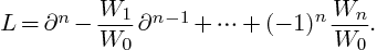
3.Factoring linear
differential operators
Let be an effective algebraically closed
subfield of . Consider a monic linear
differential operator , where .
In this section, we present an algorithm for finding a non-trivial
factorization  with
with  whenever such a factorization exists.
3.1.Factoring
and invariant subspaces under
Let be a basis of solutions for the equation
, where is  an abstract differential field. We denote the Wronskian of
by
an abstract differential field. We denote the Wronskian of
by
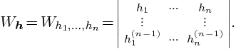
It is classical (and easy to check) that
 |
(7) |
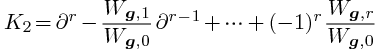
When expanding the determinant  in terms of the
matrices
in terms of the
matrices
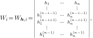
it follows that
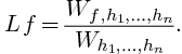
Denoting by  the logarithmic derivative of
  , it can also be checked by induction that
admits as solutions, whence  ,
using Euclidean division in the skew polynomial ring
,
using Euclidean division in the skew polynomial ring  .
.
Proposition 22.
-
If admits a factorization ,
then leaves
 invariant.
-
If
 is an invariant subvector space of , then admits a
factorization
is an invariant subvector space of , then admits a
factorization  with
with  .
.
Proof. Assume that  admits a factorization . Then, given
  and , we have
  ,
whence
,
whence  . Conversely, assume that
  is an invariant subvector space of
and let
is an invariant subvector space of
and let  be a basis of .
Then we observe that
be a basis of .
Then we observe that  for all .
Consequently,
for all .
Consequently,
for all , so that  , by
corollary 3. Hence
, by
corollary 3. Hence
 |
(8) |
is a differential operator with coefficients in

which vanishes on
. But this is only possible
if

divides
.
3.2.A lemma from linear algebra
Lemma 23. Let  be a non-unitary algebra of nilpotent matrices in
  .
Then there exists a basis of in which is lower triangular for all
.
Then there exists a basis of in which is lower triangular for all  .
.
Proof. Let be a matrix
such that  is a non-zero vector space of
minimal dimension. Given
is a non-zero vector space of
minimal dimension. Given  and
and  ,
we claim that
,
we claim that  . Assume the contrary, so that
 . By the minimality hypothesis, we must have
 . In particular,
  and
and
 . Again by the minimality hypothesis, it
follows that
. Again by the minimality hypothesis, it
follows that  . In other words, the restriction
of
. In other words, the restriction
of  to is an
isomorphism on . Hence
admits a non-zero eigenvector in , which
contradicts the fact that is nilpotent.
to is an
isomorphism on . Hence
admits a non-zero eigenvector in , which
contradicts the fact that is nilpotent.
Let us now prove the lemma by induction over

.
If

or

, then we have
nothing to do, so assume that

and

. We claim that
admits a
non-trivial invariant subvector space

.
Indeed, we may take

if

and

if

. Now consider
a basis
of
and
complete it to a basis

of
.
Then each matrix in
is lower triangular with
respect to this basis. Let

and

be the algebras of lower dimensional matrices which
occur as upper left
resp. lower right blocks of
matrices in
. We conclude by applying the
induction hypothesis on
and
.
Let be a finite set of non-zero nilpotent
matrices. If all matrices in the -algebra  generated by are nilpotent,
then it is easy to compute a basis for which all matrices in are lower triangular. Indeed, setting
generated by are nilpotent,
then it is easy to compute a basis for which all matrices in are lower triangular. Indeed, setting  for all , we first compute a basis of
  . We successively complete this basis into a basis of ,
  and so on until
  .
.
If not all matrices in are nilpotent, then the
proof of lemma 23 indicates a method for the computation of
a matrix in which is not nilpotent. Indeed, we
start by picking an  and set
  ,
where is smallest with
,
where is smallest with  .
We next set
.
We next set  and iterate the following loop. Take
a matrix
and iterate the following loop. Take
a matrix  and distinguish the following three
cases:
and distinguish the following three
cases:
-
-
Set
 and continue.
-
-
Set
 ,
,  and continue.
-
-
Return the non-nilpotent matrix
 .
.
At the end of our loop, we either found a non-nilpotent matrix, or we
have  for all
  . In the
second case, we obtain a non-trivial invariant subspace of as in the proof of lemma 23 and we
recursively apply the algorithm on this subspace and a complement. In
fact, the returned matrix is not even monopotent
(i.e. not of the form
. In the
second case, we obtain a non-trivial invariant subspace of as in the proof of lemma 23 and we
recursively apply the algorithm on this subspace and a complement. In
fact, the returned matrix is not even monopotent
(i.e. not of the form  , where
  is a nilpotent matrix), since it both admits zero and
a non-zero number as eigenvalues.
is a nilpotent matrix), since it both admits zero and
a non-zero number as eigenvalues.
3.3.Computation of non-trivial
invariant subspaces
Proposition 22 in combination with theorem 20
implies that the factorization of linear differential operators in reduces to the computation of non-trivial invariant
subvector spaces under the action of  whenever
they exist.
whenever
they exist.
In this section, we will first solve a slightly simpler problem:
assuming that is an effective algebraically
closed field and given a finite set of matrices  ,
we will show how to compute a non-trivial invariant subspace of under the action of , whenever such a exists.
,
we will show how to compute a non-trivial invariant subspace of under the action of , whenever such a exists.
Good candidate vectors
Given
a vector it is easy to compute the smallest
subspace  of which is
invariant under the action of and which contains
. Indeed, starting with a basis
of which is
invariant under the action of and which contains
. Indeed, starting with a basis  ,
we keep enlarging
,
we keep enlarging  with elements in
  until saturation. Since will never
contain more than elements, this algorithm
terminates. A candidate vector for
generating a non-trivial invariant subspace of
is said to be good if
until saturation. Since will never
contain more than elements, this algorithm
terminates. A candidate vector for
generating a non-trivial invariant subspace of
is said to be good if  .
.
The -algebra generated by
We notice that  is an
invariant subspace for , if and only if is an invariant subspace for the -algebra
is an
invariant subspace for , if and only if is an invariant subspace for the -algebra
 generated by . Again it
is easy to compute a basis for . We start with a
basis of
generated by . Again it
is easy to compute a basis for . We start with a
basis of  and keep
adjoining elements in
and keep
adjoining elements in  to
until saturation. We will avoid the explicit basis of ,
which may contain as much as
to
until saturation. We will avoid the explicit basis of ,
which may contain as much as  elements, and
rather focus on the efficient computation of good candidate vectors.
elements, and
rather focus on the efficient computation of good candidate vectors.
-splittings
A decomposition
 , where
  are non-empty
vector spaces, will be called an -splitting
of , if the projections
are non-empty
vector spaces, will be called an -splitting
of , if the projections  of on
of on  are all in . Then, given , we have
  if and only if
  for all
  . If we choose a basis for
which is a union of bases for the , we notice
that the
. If we choose a basis for
which is a union of bases for the , we notice
that the  are
are  block
matrices. In the above algorithm for computing the -algebra
generated by it now suffices to compute with
block matrices of this form. In particular, the computed basis of will consist of such matrices. The trivial
decomposition
block
matrices. In the above algorithm for computing the -algebra
generated by it now suffices to compute with
block matrices of this form. In particular, the computed basis of will consist of such matrices. The trivial
decomposition  is clearly an -splitting.
Given
is clearly an -splitting.
Given  , we notice that any
  -splitting
is also an -splitting.
-splitting
is also an -splitting.
Refining -splittings
An -splitting  is said to be
finer than the -splitting if is a direct sum of a subset of
the
is said to be
finer than the -splitting if is a direct sum of a subset of
the  for each . Given an
-splitting and an arbitrary element , we may
obtain a finer -splitting w.r.t
as follows. Let
for each . Given an
-splitting and an arbitrary element , we may
obtain a finer -splitting w.r.t
as follows. Let  and
consider
and
consider  . If
. If  are the
eigenvalues of
are the
eigenvalues of  , then
  is
an
is
an  -splitting of , where
 . Collecting these -splittings,
we obtain a finer -splitting
. Collecting these -splittings,
we obtain a finer -splitting  of . This -splitting,
which is said to be refined w.r.t. ,
has the property that
of . This -splitting,
which is said to be refined w.r.t. ,
has the property that  is monopotent on
  for each , with unique eigenvalue
 .
.
We now have the following algorithm for computing non-trivial -invariant subspaces of when they
exist.
Algorithm Invariant_subspace
Input: a set of non-zero matrices in
Output: an -invariant
subspace of or fail
Step 1. [Initial -splitting]
Compute a “random non-zero element”  of
of 
Step 2. [One dimensional components]
If  for all
then return fail
for all
then return fail
Step 3. [Higher dimensional components]
Let be such that 
Let 
Let 
If  then go to step 4 and otherwise to
step 5
then go to step 4 and otherwise to
step 5
Step 4. [Non-triangular case]
Let  be non-monopotent on (cf. previous section)
Refine the -splitting
w.r.t. and return to step
2
Step 5. [Potentially triangular case]
Choose  and compute
Otherwise, set  and repeat step 5
The algorithm needs a few additional explanations. In step  , we may take to be an arbitrary
element in . However, it is better to take a
“small random expression in the elements of ”
for . With high probability, this yields an -splitting which will not need to be refined in the
sequel. Indeed, the subset of matrices in which
yield non-maximal -splittings is a closed
algebraic subset of measure zero, since it is determined by coinciding
eigenvalues. In particular, given an -splitting
w.r.t. , it
will usually suffice to check that each is
monopotent on each , in order to obtain an -splitting w.r.t. the other elements in
.
, we may take to be an arbitrary
element in . However, it is better to take a
“small random expression in the elements of ”
for . With high probability, this yields an -splitting which will not need to be refined in the
sequel. Indeed, the subset of matrices in which
yield non-maximal -splittings is a closed
algebraic subset of measure zero, since it is determined by coinciding
eigenvalues. In particular, given an -splitting
w.r.t. , it
will usually suffice to check that each is
monopotent on each , in order to obtain an -splitting w.r.t. the other elements in
.
Throughout the algorithm, the -splitting gets
finer and finer, so the -splitting ultimately
remains constant. From this point on, the space  can only strictly decrease in step
  , so also remains constant, ultimately. But then we either find
a non-trivial invariant subspace in step 5, or all components of the
-splitting become one-dimensional. In the latter
case, we either obtain a non-trivial invariant subspace in step 1, or a
proof that
, so also remains constant, ultimately. But then we either find
a non-trivial invariant subspace in step 5, or all components of the
-splitting become one-dimensional. In the latter
case, we either obtain a non-trivial invariant subspace in step 1, or a
proof that  for every
  (and thus for every
  ).
).
Remark 24. Assume that
is no longer an effective algebraically closed field, but rather a field
with an approximate zero-test. In that case, we
recall that a number which is approximately zero is not necessarily
zero. On the other hand, a number which is not approximately zero is
surely non-zero. Consequently, in our algorithm for the
computation of  , the dimension of can be too small, but it is never too large. In
particular, if the algorithm Invariant_subspace fails,
then the approximate proof that
, the dimension of can be too small, but it is never too large. In
particular, if the algorithm Invariant_subspace fails,
then the approximate proof that  for every yields a genuine proof that there are no non-trivial
invariant subspaces.
for every yields a genuine proof that there are no non-trivial
invariant subspaces.
3.4.Factoring linear
differential operators
Putting together the results from the previous sections, we now have the
following algorithm for finding a right factor of .
Algorithm Right_factor
Input: 
Output: a non-trivial right-factor of or fail
Step 1. [Compute generators]
Choose and let 
Compute a finite set  of generators for
(cf. theorem 20)
of generators for
(cf. theorem 20)
Step 2. [Initial precision]
Step 3. [Produce invariant subspace]
Let 
If  then return fail
Let  be a column basis of
Let 
Step 4. [Produce and check guess]
Let 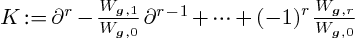
Return 
Step 5. [Increase precision]
The main idea behind the algorithm is to use proposition 22
in combination with Invariant_subspace so as to provide
good candidate right factors of in  . Using reconstruction of coefficients in
  from Laurent series in
  with increasing
precisions, we next produce good candidate right factors in . We keep increasing the precision until we find a right
factor or a proof that is irreducible. Let us
detail the different steps a bit more:
with increasing
precisions, we next produce good candidate right factors in . We keep increasing the precision until we find a right
factor or a proof that is irreducible. Let us
detail the different steps a bit more:
-
Step 2
-
We will work with power series approximations of
 terms and approximate zero-tests in . The
degree of a rational function
terms and approximate zero-tests in . The
degree of a rational function  is defined by
 . The initial precisions
and
. The initial precisions
and  have been chosen as small as possible.
Indeed, we want to take advantage of a possible quick answer when
computing with a small precision (see also the explanations below of
step 5).
have been chosen as small as possible.
Indeed, we want to take advantage of a possible quick answer when
computing with a small precision (see also the explanations below of
step 5).
-
Step 3
-
If Invariant_subspace fails, then there exists no
factorization of , by remark 24.
Effective power series and Laurent series are defined in a similar way
as effective real numbers (in particular, we don't assume the
existence of an effective zero-test). Efficient algorithm for such
computations are described in [vdH02].
-
Step 4
-
The reconstruction of
 and
and  from
from  and
and  contains two
ingredients: we use Padé approximation to find rational
function approximations of degree
contains two
ingredients: we use Padé approximation to find rational
function approximations of degree  and the
LLL-algorithm to approximate numbers by
numbers in .
and the
LLL-algorithm to approximate numbers by
numbers in .
-
Step 5
-
Doubling the precision at successive steps heuristically causes the
computation time to increase geometrically at each step. In
particular, unsuccessful computations at lower precisions don't take
much time with respect to the last successful computation with respect
to the required precision. Instead of multiplying the precisions by
two, we also notice that it would be even better to increase by a
factor which doubles the estimated computation time at each step. Of
course, this would require a more precise complexity analysis of the
algorithm.
The problem of reconstructing elements in from
elements in is an interesting topic on its own.
In theory, one may consider the polynomial algebra over  generated by all coefficients occurring in and
the number we wish to reconstruct. We may then
apply the LLL-algorithm [LLL82] on the lattice spanned by
generated by all coefficients occurring in and
the number we wish to reconstruct. We may then
apply the LLL-algorithm [LLL82] on the lattice spanned by
 monomials of smallest total degree (for
instance) and search for minimal
monomials of smallest total degree (for
instance) and search for minimal  -digit
relations. If is the algebraic closure of , then we may simply use the lattice spanned by the
first powers of .
-digit
relations. If is the algebraic closure of , then we may simply use the lattice spanned by the
first powers of .
At a sufficiently large precision , the
LLL-algorithm will ultimately succeed for all coefficients of a
candidate factorization which need to be reconstructed. If there are no
factorizations, then the algorithm will ultimately fail at step 3. This
proofs the termination of Right_factor.
Remark 25. In practice, and especially if  , it would be nice to use more of the structure of the
original problem. For instance, a factorization of
actually yields relations on the coefficients which we may try to use.
For high precision computations, it is also recommended to speed the
LLL-algorithm up using a similar dichotomic algorithm as for fast
g.c.d. computations [Moe73, PW02].
, it would be nice to use more of the structure of the
original problem. For instance, a factorization of
actually yields relations on the coefficients which we may try to use.
For high precision computations, it is also recommended to speed the
LLL-algorithm up using a similar dichotomic algorithm as for fast
g.c.d. computations [Moe73, PW02].
Remark 26. Notice that we did not use bounds for
the degrees of coefficients of possible factors in our algorithm. If a
bound  is available, using techniques from [BB85, vH97, vdPS03], then one may
take
is available, using techniques from [BB85, vH97, vdPS03], then one may
take  instead of
  in step
5. Of course, bounds for the required precision
in step
5. Of course, bounds for the required precision  are even harder to obtain. See [BB85] for some results in
that direction.
are even harder to obtain. See [BB85] for some results in
that direction.
4.Computing differential
Galois groups
4.1.Introduction
Throughout this section,  will stand for the
field of effective complex number with the
approximate zero-test at precision
will stand for the
field of effective complex number with the
approximate zero-test at precision  . This field
has the following properties:
. This field
has the following properties:
-
EH1
-
We have an effective zero-test in .
-
EH2
-
There exists an algorithm which takes on input
 and which computes a finite set of generators for the -vector
space of integers
and which computes a finite set of generators for the -vector
space of integers  with
with  .
.
-
EH3
-
There exists an algorithm which takes on input
 and which computes a finite set of generators for the -vector
space of integers with
and which computes a finite set of generators for the -vector
space of integers with  .
.
-
EH4
-
is closed under exponentiation and logarithm.
Indeed, we obtain EH2 and EH3 using
the LLL-algorithm. Some of the results in this section go through when
only a subset of the conditions are satisfied. In that case, we notice
that EH2 EH1,
EH3EH1 and
EH4(EH2
EH1,
EH3EH1 and
EH4(EH2 EH3).
EH3).
Given a finite set of matrices  , we give a
numerical algorithm for the computation of the smallest closed algebraic
subgroup
, we give a
numerical algorithm for the computation of the smallest closed algebraic
subgroup  of
of  which
contains . We will represent
by a finite set
which
contains . We will represent
by a finite set  and the finite basis
  of a Lie algebra over , such that

and each  corresponds to a unique connected
component
corresponds to a unique connected
component  of . We will
also prove that there exists a precision
of . We will
also prove that there exists a precision  such
that the algorithm yields the theoretically correct result for all
such
that the algorithm yields the theoretically correct result for all  .
.
4.2.The algebraic group generated by
a diagonal matrix
Let  be the group of invertible diagonal
matrices. Each matrix has the form
be the group of invertible diagonal
matrices. Each matrix has the form  , where
  is the vector in
  of the elements on the diagonal of .
The coordinate ring
of the elements on the diagonal of .
The coordinate ring  of
is the set
of
is the set  of Laurent polynomials in .
Now consider the case when consists of a single
diagonal matrix  . Let
. Let  be
the ideal which defines
be
the ideal which defines  . Given a relation
  between the
  , any power
  satisfies the same relation
  ,
whence
,
whence  . Let
. Let  be the ideal
generated by all
be the ideal
generated by all  , such that
  .
.
Lemma 27. We have  .
.
Proof. We already observed that  .
Assuming for contradiction that
.
Assuming for contradiction that  , choose
such that

is minimal. If

,
then

, since otherwise

and
has less than
terms. In particular, the vectors
with
are linearly independent. But this contradicts
the fact that
for all
.
By EH2, we may compute a minimal finite set  of generators for the -vector space
of with . We may also
compute a basis for
of generators for the -vector space
of with . We may also
compute a basis for  ,
where
,
where  . Then
  is the
connected component of
is the
connected component of  , since
  for all , and cannot be
further enlarged while conserving this property.
for all , and cannot be
further enlarged while conserving this property.
Let  . We construct a basis
  of
of  , by taking
  to be
shortest in
to be
shortest in  (if
(if  ) or (if
  ), such that
  . This basis determines a toric change of coordinates
  with
with  such that
  with respect to the new coordinates. Similarly, we may
construct a basis
with respect to the new coordinates. Similarly, we may
construct a basis  of
of  , by
taking each
, by
taking each  to be shortest in
  such that
  is maximal. This basis determines a
second toric change of coordinates
is maximal. This basis determines a
second toric change of coordinates  with
with  such that
  (
( )
with respect to the new coordinates.
)
with respect to the new coordinates.
After the above changes of coordinates, the ideal
is determined by the equations  . Setting

it follows that  . Rewriting
with respect to the original coordinates now completes the computation
of .
. Rewriting
with respect to the original coordinates now completes the computation
of .
4.3.The algebraic group generated by
a single matrix
Let us now consider the case when consists of a
single arbitrary matrix . Then we first compute
the multiplicative Jordan decomposition of .
Modulo a change of basis of  , this means that
where  and
and  are the
semi-simple and unipotent parts of :
are the
semi-simple and unipotent parts of :
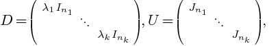
where
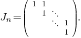
Proposition 28. We have 
Remark. Notice that  is
well-defined for power series
is
well-defined for power series  and nilpotent
matrices
and nilpotent
matrices  ; in this case,
  and
and  .
.
Proof. The assertion is clear if

, so assume

. Let

.
We clearly have

, since

is a closed algebraic group which contains

.
Moreover, the set
is infinite, so
. Since
is irreducible and

, we conclude that

.
Proposition 29. We have  .
.
Proof. Since

is a
commutative group, [
Hum81, Theorem 15.5] implies that
, where
and
are closed subgroups of
. Now

and

are closed
subgroups of
 resp.
resp. 
, so

is a closed subgroup of
. Since
, it follows that
.
Corollary 30. If  , then
 .
.
4.4.Membership testing
for the connected component
In order to compute the closure of the product of a finite number of
algebraic groups of the form  , an important
subproblem is to test whether a given matrix
, an important
subproblem is to test whether a given matrix  belongs to
  .
.
We first observe that  implies
  .
After the computation of
.
After the computation of  and
and  with
with  it therefore suffices to check that
  and
and  . In fact, it suffices to
check whether
. In fact, it suffices to
check whether  , where
  is
the unique matrix in with
is
the unique matrix in with  .
Modulo a suitable base change, we have thus reduced the general problem
to the case when is a diagonal matrix whose
eigenvalues are all roots of unity.
.
Modulo a suitable base change, we have thus reduced the general problem
to the case when is a diagonal matrix whose
eigenvalues are all roots of unity.
Assume that and  are such
that
are such
that  . Since and
  commute, it follows that and
can be diagonalized w.r.t. a common
basis. The elements of this basis are elements of the different
eigenspaces of . In other words, if
commute, it follows that and
can be diagonalized w.r.t. a common
basis. The elements of this basis are elements of the different
eigenspaces of . In other words, if  with pairwise distinct , then
  is diagonal for some block matrix
  with
with  for each . It
follows that
for each . It
follows that  for certain
  .
Without loss of generality, we may therefore replace
by the intersection of with
.
Without loss of generality, we may therefore replace
by the intersection of with  .
.
From now on, we assume that the above two reductions have been made. Let
 be a diagonal matrix in .
By lemma 27, we have if and only if
any -linear relation
be a diagonal matrix in .
By lemma 27, we have if and only if
any -linear relation  induces a relation
  , where
  .
Now consider a random matrix
.
Now consider a random matrix  in ,
i.e. a linear combination of the basis elements with small
random integer coefficients. We compute its blockwise Jordan normal form
in ,
i.e. a linear combination of the basis elements with small
random integer coefficients. We compute its blockwise Jordan normal form
 so that
  and let be the restriction of
  to the
diagonal. We have
to the
diagonal. We have  . Computing a basis for the
-linear relations of the form
using EH3, the above criterion now enables us to check
whether
. Computing a basis for the
-linear relations of the form
using EH3, the above criterion now enables us to check
whether  .
.
If the check whether succeeds, then we are
clearly done. Otherwise, since was chosen in a
random way, the relation  is very likely to be
satisfied for all possible choices of
is very likely to be
satisfied for all possible choices of  (up to
permutations of coordinates inside each block). Indeed, the for which this is not the case lie on a countable union
(up to
permutations of coordinates inside each block). Indeed, the for which this is not the case lie on a countable union
 of algebraic variety of a lower dimension, so
has measure .
Heuristically speaking, we may therefore conclude that
of algebraic variety of a lower dimension, so
has measure .
Heuristically speaking, we may therefore conclude that  if the check fails (at least temporarily, modulo some final checks when
the overall computation of
if the check fails (at least temporarily, modulo some final checks when
the overall computation of  will be completed).
Theoretically speaking, we may perform the above computations with  instead of , where is a basis of and the
  are formal parameters. We then check whether the relation
 is still satisfied for the analogue
  of . If so, then we are sure that
. Otherwise, we keep trying with other random
elements of .
of . If so, then we are sure that
. Otherwise, we keep trying with other random
elements of .
It is likely that a more efficient theoretical algorithm can be designed
for testing -linear relations between the
eigenvalues of elements in . One of the referees
suggested to use similar methods as in [Mas88, Ber95,
CS98]. However, we did not study this topic in more detail,
since our final algorithm for the computation of Galois groups will be
based on heuristics anyway. We also notice that a “really
good” random number generator should actually never
generate points which satisfy non-trivial algebraic relations.
4.5.Computing the closure
of
A Lie algebra is said to be algebraic,
if it is the Lie algebra of some algebraic group, i.e. if
is an algebraic subset of .
It is classical [Bor91, Corollary 7.7] that the smallest
Lie algebra generated by a finite number of algebraic Lie algebras is
again algebraic. The Lie algebras we will consider in our algorithms
will always assumed to be algebraic. Given a finite number  of algebraic Lie algebras and a basis
for
of algebraic Lie algebras and a basis
for  , it is easy to enrich
so that
, it is easy to enrich
so that  is a Lie algebra: as long as
  for two elements
  , we add
  to . By what precedes, the computed
Lie algebra is again algebraic.
to . By what precedes, the computed
Lie algebra is again algebraic.
Putting together the ingredients from the previous sections, we now have
the following algorithm for computing the smallest closed algebraic
group which contains .
Algorithm Closure()
Input: A subset  of
of 
Output: a numeric approximation of 
Step 1. [Initialize algorithm]
Compute  for each
Let  (notice that
  )
)
Let 
Step 2. [Closure]
Return
The termination of this algorithm relies on a lemma, whose proof was
kindly communicated to the author by J.-Y. Hée.
Lemma 31. Let be a
closed algebraic subgroup of  and let
  be a finite number of matrices in the normalizer of . Denote by
  the group
generated by and
the group
generated by and  . If all
elements in
. If all
elements in  have finite order, then is finite.
Proof. In the case when

,
the result is classical [
Dix71, Theorem 9.2]. In the
general case, the normalizer

of
is a closed algebraic subgroup of
and
is a normal subgroup of
.
By [
Bor91, Theorem 6.8 and Proposition 1.10], it follows
that

is an affine algebraic group which is
isomorphic to a closed algebraic matrix group. This reduces the
general case to the special case when
.
Theorem 32. There exists an  such that, for every with ,
the set returned by Closure,
considered as a subset of
such that, for every with ,
the set returned by Closure,
considered as a subset of  , coincides with the
smallest closed algebraic subgroup of which contains .
, coincides with the
smallest closed algebraic subgroup of which contains .
Proof. Clearly, the dimension of  increases throughout the execution of the algorithm, so
it remains ultimately constant. At this point, the set will keep growing and the lemma implies that ultimately stabilizes. When this happens, is closed under multiplication modulo ,
as well as under multiplicative inverses, since each element in has finite order modulo . We
conclude that is indeed the smallest closed
algebraic subgroup of which contains , provided that the approximate zero-test always returns
the right result.
increases throughout the execution of the algorithm, so
it remains ultimately constant. At this point, the set will keep growing and the lemma implies that ultimately stabilizes. When this happens, is closed under multiplication modulo ,
as well as under multiplicative inverses, since each element in has finite order modulo . We
conclude that is indeed the smallest closed
algebraic subgroup of which contains , provided that the approximate zero-test always returns
the right result.
In order to prove the correctness at a sufficient precision, we
assume that we use the theoretic membership test from section
4.4 and that the random number generator successively
generates the same random numbers each time we relaunch the
algorithm at a higher precision. Now consider the trace of the
execution of our algorithm when using an infinite precision. Let
be a sufficient precision such that all
zero-tests in this execution tree are still correct when we replace
the infinite precision by a precision
. Then
the trace of the execution any finite precision
coincides with the trace of the execution at infinite precision.
This completes the proof.

Remark 33. The main improvement of the algorithm
Closure w.r.t. the algorithm from [DJK03]
lies in the more efficient treatment of the connected component (using
linear algebra). On the other hand, the mere enumeration of
representatives in each connected component can be very unefficient
(although a Gröbner basis might be of the same size). Fortunately,
we will see in the next sections how to remove this drawback.
Assume now that is the set of generators for
as computed in theorem 20. Assume
that we have computed a reasonable candidate for
, expressed in the original basis corresponding
to . We still have to reconstruct  and
and 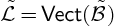 with
with  such that
  .
.
In the case of  , by selecting a suitable basis of
 , we may consider as a
big
, we may consider as a
big  matrix whose first
columns are linearly independent. We compute the row-echelon form of
this basis:
matrix whose first
columns are linearly independent. We compute the row-echelon form of
this basis:
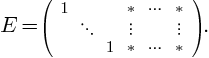
The entries of  must be in :
provided that is indeed generated by a basis of
matrices with entries in , the row-echelon form
of this second basis coincides with . It
therefore suffices to reconstruct the entries of
using the LLL-algorithm.
must be in :
provided that is indeed generated by a basis of
matrices with entries in , the row-echelon form
of this second basis coincides with . It
therefore suffices to reconstruct the entries of
using the LLL-algorithm.
In the case of a matrix  , the set
  is an algebraic variety of dimension
over . Now choose
is an algebraic variety of dimension
over . Now choose  close
to in such a way that
independent coordinates of
close
to in such a way that
independent coordinates of  are all in
  . Then the other coordinates of ,
considered as elements of , are easily found
using Newton's method. Since is an algebraic
variety, these other coordinates are actually in ,
and we reconstruct them using the LLL-algorithm.
. Then the other coordinates of ,
considered as elements of , are easily found
using Newton's method. Since is an algebraic
variety, these other coordinates are actually in ,
and we reconstruct them using the LLL-algorithm.
4.6.Fast computations with the
connected components
The algorithm Closure from the previous section is quite
inefficient when the set becomes large. It is
therefore useful to seek for a better computational representation of
. For finite groups , one
classical idea is to search for a sequence of subgroups
 |
(9) |
such that the indices  are small. Then we may
represent elements in by sequences
are small. Then we may
represent elements in by sequences  with
with  for each .
This representation is particularly useful if
operates on a set
for each .
This representation is particularly useful if
operates on a set  and if there exists points
 in such that
is the stabilizer of the set  for each . Then the set
  corresponds to the
orbit of
corresponds to the
orbit of  while leaving
  fixed [Sim70, Sim71].
In the case of matrix groups, one often takes
for [MO95]. However, this approach
only yields interesting results when there exist non-trivial invariant
subspaces under the action of the group, which will usually not be the
case for us (otherwise we may factor and
consider smaller problems). A theoretical way out of this is to also
consider the action of on exterior powers  . However, this approach is very expensive from a
computational point of view. In our more specific context of matrices
with complex entries, we will therefore combine two other approaches:
non-commutative lattice reduction and the operation of
on
. However, this approach is very expensive from a
computational point of view. In our more specific context of matrices
with complex entries, we will therefore combine two other approaches:
non-commutative lattice reduction and the operation of
on  via conjugations
  .
.
The algebra admits a natural (multiplicative)
norm, given by

where  stands for the Euclidean norm on . If
  is finite, this enables us to
construct
is finite, this enables us to
construct  as in (9) as follows.
Assuming that
as in (9) as follows.
Assuming that  have been constructed, we consider
a matrix
have been constructed, we consider
a matrix  for which
  is
minimal, and let
is
minimal, and let  be the set generated by
  and
and  in .
This construction allows us to rapidly identify a big commutative part
of . More precisely, we have
in .
This construction allows us to rapidly identify a big commutative part
of . More precisely, we have
Proposition 34. Let  be such that
  and
and  . Then we have

Proof. Writing  and
and  , we expand
  and
and  in
in  . This yields a
non-commutative power series in
. This yields a
non-commutative power series in  and
and  whose terms in
  and vanish. It follows that
The proposition implies that  whenever
  . Now take
  and
and  with
with  , where the are as
above. Then it follows that
, where the are as
above. Then it follows that  and
and  commute whenever
  . What is more, proposition 34 shows that taking commutators is a convenient way to
construct matrices close to identity from a set of non-commutative
generators.
. What is more, proposition 34 shows that taking commutators is a convenient way to
construct matrices close to identity from a set of non-commutative
generators.
However, from the effective point of view, we will not compute the
exact computation of minimal representatives
in cosets of algebraic groups in detail. We will rather simulate such a
computation in a way which is sufficient for our purpose. If is such that  is small, then we
will also try to use the fact that the centralizer
is small, then we
will also try to use the fact that the centralizer  of is often a big subgroup of
  ,
so the orbit of
,
so the orbit of  is small.
4.7.Non-commutative lattice
reduction
Let be a closed algebraic subgroup of with associated Lie-algebra . In
this section, we will show how to compute efficiently with elements of
the finite group  . Until the very end of this
section, we assume that is included in the
connected component of the normalizer of in . We denote by
. Until the very end of this
section, we assume that is included in the
connected component of the normalizer of in . We denote by  the Lie algebra
of this connected component. By [Hum81, Theorem 13.3], we
have
the Lie algebra
of this connected component. By [Hum81, Theorem 13.3], we
have  .
.
Orthogonal projection
Let  and
recall that belongs to the normalizer of . If
and
recall that belongs to the normalizer of . If  , then
  also belongs to the normalizer of . Since
  lies in the connected component of this normalizer,
we have
lies in the connected component of this normalizer,
we have  . Now consider the orthogonal supplement
 of for the Hermitian
product on . We define
of for the Hermitian
product on . We define  ,
where
,
where  is the orthogonal projection of
  on . From
  ,
it follows that
,
it follows that  , and we denote
  .
Since
.
Since  is connected, the function
  may actually be analytically continued to a multivalued
function
may actually be analytically continued to a multivalued
function  . After choosing branch cuts (the way
this is done is not crucial for what follows, provided that we make the
standard choice for with ),
this allows us to extend the definitions of
. After choosing branch cuts (the way
this is done is not crucial for what follows, provided that we make the
standard choice for with ),
this allows us to extend the definitions of  and
and
 to the case when
  .
.
Representation of the elements in
Let
and  be such that
-
 .
.
-
 generates
  .
.
-
 whenever
  is another
such generator.
is another
such generator.
Let  be the prime-decomposition of the order of
modulo , with
be the prime-decomposition of the order of
modulo , with  . Let
. Let  and
and  for all
  . Let
. Let  be the
subgroup of of elements which commute with
be the
subgroup of of elements which commute with  modulo , so that
  . For
. For  , we represent elements in the
quotient
, we represent elements in the
quotient  by elements in the orbit of the action
 modulo
  . Since , the set
  is a Lie algebra whose
normalizer contains
is a Lie algebra whose
normalizer contains  . Consequently,
  , and we represent elements in by
products
, and we represent elements in by
products  , with
  and
and  . The elements in
  are
represented in a similar way as the elements in ,
using recursion. The successive matrices for
, , etc. will
be called a basis for . A basis
are
represented in a similar way as the elements in ,
using recursion. The successive matrices for
, , etc. will
be called a basis for . A basis  is said to be sorted if
  .
.
Adding new elements to a basis
Let
be a sorted basis for and assume that we want to
compute the extension  of
by a new matrix . Whenever we hit an element
of
by a new matrix . Whenever we hit an element  with
with  during our computations,
then we start the process of basis reduction, which is described below.
Whenever we find an element in
during our computations,
then we start the process of basis reduction, which is described below.
Whenever we find an element in  , then we abort
all computations and return this element (indeed, in that case, we may
continue with the closure of the connected component in Closure).
, then we abort
all computations and return this element (indeed, in that case, we may
continue with the closure of the connected component in Closure).
Let  , , etc.
be as above. We start by computing the orbit of
, , etc.
be as above. We start by computing the orbit of  modulo
  for
for  . Whenever we
hit an element
. Whenever we
hit an element  (modulo )
with
(modulo )
with  or
or  , then we start
the process of basis reduction. Otherwise, we obtain a finite orbit,
together with a finite number of matrices by which we have to extend
. We keep doing this using the same method for
until
, then we start
the process of basis reduction. Otherwise, we obtain a finite orbit,
together with a finite number of matrices by which we have to extend
. We keep doing this using the same method for
until  .
.
At the end, we still have to show how to extend
with a new matrix  . Now recursive application of
the algorithm to
. Now recursive application of
the algorithm to  and
yields a sorted basis
and
yields a sorted basis  . When keeping track of the
corresponding powers of
. When keeping track of the
corresponding powers of  during the computations,
we also obtain a finite system of generators for
during the computations,
we also obtain a finite system of generators for  .
Using g.c.d. computations we either obtain a minimal
generator
.
Using g.c.d. computations we either obtain a minimal
generator  or a new element in the connected
component. In the first case, we return
or a new element in the connected
component. In the first case, we return  if
if  and apply basis reduction otherwise.
Basis reduction
Let  be in
with . We call a raw basis. In the above algorithms, raw bases
occur when we are given an ordered basis
be in
with . We call a raw basis. In the above algorithms, raw bases
occur when we are given an ordered basis  for
, and we find a new element
for
, and we find a new element  with
with  .
.
Using the above base extension procedure, we may transform a raw basis
 into a basis for :
starting with
into a basis for :
starting with  , we successively add
  . However, it is more efficient to reduce
first. More precisely, let us now describe a procedure which tries to
replace by a better raw basis
. However, it is more efficient to reduce
first. More precisely, let us now describe a procedure which tries to
replace by a better raw basis  ,
with
,
with  , and whose elements are closer to identity.
Of course, we may always return the original basis if a better one could
not be found.
, and whose elements are closer to identity.
Of course, we may always return the original basis if a better one could
not be found.
We first test whether all basis elements are roots of unity modulo . If not, then we found a new element in the connected
component. We next test whether there exist with
 , in which case we keep adding the smallest such
commutator to the basis. Whenever this stops, we write
, in which case we keep adding the smallest such
commutator to the basis. Whenever this stops, we write  with
with  and consider all lattice reductions
  proposed by the LLL-algorithm in the commutative
vector space . Whenever
proposed by the LLL-algorithm in the commutative
vector space . Whenever  ,
for one such reduction, then we perform the corresponding reduction
,
for one such reduction, then we perform the corresponding reduction  on our basis and keep repeating the basis reduction
process.
on our basis and keep repeating the basis reduction
process.
The general case
We still have to show how to deal
with the case when is not included in the
connected component of the normalizer of in . In that case, we start
with the computation of a basis for , using
linear algebra. Since  is a normal subgroup of
, we have
is a normal subgroup of
, we have  . Now we have
explained above how to compute with elements in .
If
. Now we have
explained above how to compute with elements in .
If  , then may use recursion for computations in
the finite group
, then may use recursion for computations in
the finite group  . If
. If  ,
then elements in have necessarily small order,
so we simply list the elements of .
,
then elements in have necessarily small order,
so we simply list the elements of .
5.Conclusion and final notes
We hope that we provided convincing evidence that analytic methods may
be used for the efficient computation of differential Galois groups and
related problems like the factorization of linear differential
operators.
The two main remaining challenges are the concrete implementation of the
algorithms presented here (as part of a more general library for the
computation with analytic functions such as [vdHea05]) and
the development of a priori or a posteriori methods
for ensuring the correctness of the computed result. Some ideas into
this direction are as follows:
-
Use theoretical bounds on the number of connected components of the
computed Galois group and related bounds on the sizes of the basis
elements in EH2 and EH3. See [DJK03, Section 3.2] for some results.
-
Use the classification theory for algebraic groups in order to gather
more information about the computed Galois group .
In particular, it is useful to compute the radical (or unipotent
radical) of , thereby reducing the study of
to the study of a finite group, a semisimple
(or reductive) group and a solvable (or unipotent) group [Hum81,
page 125]. We refer to [dG00] for computational aspects
of the corresponding Lie algebras.
-
Use the classical theory of invariant subspaces in symmetric products
or exterior powers as an a posteriori correctness check and
search for an effective version of Chevalley's theorem [Hum81,
Theorem 11.2]. One may start with generalizing [vHW97, CS98] and notice that a better knowledge of the Galois group
helps to further restrict the number of
monomials (i.e. “generalized exponents”) to
be considered. Indeed, if is an arbitrary
algebraic subgroup of , for which the ring of
invariants is easy to compute, then the invariants for must be searched in this ring. Also, their are known
algorithms for computing the invariants for certain types of algebraic
groups, like linearly reductive groups [Der99].
-
The representation for algebraic groups we
used in section 4 is efficient for computations (we
merely do linear algebra in dimension , lattice
reduction and computations with small finite groups). Nevertheless, it
may be interesting to reconstruct the algebraic equations for and search for equations which are particularly
sparse with respect to suitably chosen coordinates. For instance, a
big cyclic group admits a particularly nice (resp. large)
Gröbner basis w.r.t. well chosen (resp.
badly chosen) coordinates. Conversely, it may be interesting to switch
back from a Gröbner basis representation to our representation.
-
Carefully identify those parts of the algorithm which either prove or
disprove certain matrices to belong to the Galois group. For instance,
we know that all Stokes matrices are unipotent. Given a non-zero
transcendental number
 , we may then reliably
conclude that a Stokes matrix of the form
, we may then reliably
conclude that a Stokes matrix of the form  generates the group
 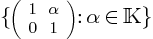 .
.
-
An interesting idea to get rid of the transcendental part of the
computations might be to quotient the values of the functions in our
basis of solutions by the action of the Galois
group. For instance, if and
are close regular points in , is it true that
the orbit of
 under the action of the Galois
group necessarily contains a point in ? This is
clearly the case for finite Galois groups and the full Galois group,
as well as for the equations
under the action of the Galois
group necessarily contains a point in ? This is
clearly the case for finite Galois groups and the full Galois group,
as well as for the equations  and
and  . More generally, as soon as
becomes more transcendental, its orbit under the action of the Galois
group becomes larger, so the likelihood of finding a point in the
intersection with increases.
. More generally, as soon as
becomes more transcendental, its orbit under the action of the Galois
group becomes larger, so the likelihood of finding a point in the
intersection with increases.
Besides the above ideas for improving the algorithms, this paper also
raises a few other interesting questions:
-
Are there more efficient approaches for the reconstruction of elements
in in section 3.4, both in the
cases when and when is
more general? Also, as pointed out above, we may want to reconstruct
equations for from the variety.
-
Does there exists an efficient membership test in section 4.4
which does not rely on probabilistic arguments?
-
Can the approach of section 4 be adapted to the
computation of a “basis” for the usual topological closure
of a finitely generated matrix group?
Of course, a better mastering of the algorithms in this paper may also
lead to more efficient algorithms for other computations which rely on
differential Galois theory, like the computation of Liouvillian or other
forms of solutions. More generally, our algorithms may be used for other
computations with algebraic matrix groups over
and other fields of characteristic . We also
expect all results to generalize to holonomic systems of linear partial
differential equations.
Acknowledgment
The author would like to thank
J.-Y. Hée, W. de Graaf, F.
Zara, J. Écalle and the referees for several helpful
comments and references.
Bibliography
-
[BB85] D. Bertrand and F. Beukers.
équations différentielles linéaires et
majorations de multiplicités. Ann. Sci. de
l'École Norm. Sup., 28(4-5):473–494, 1985.
[Bek94] E. Beke. Die
Irreduzibilität der homogenen linearen
Differentialgleichungen. Math. Ann., 45, 1894.
[Ber95] D. Bertrand. Minimal
heights and polarizations on group varieties. Duke Math.
J., 80(1):223–250, 1995.
[Bor91] A. Borel. Linear
algebraic groups. Springer-Verlag, 2nd edition, 1991.
[Bra91] B.L.J. Braaksma.
Multisummability and Stokes multipliers of linear meromorphic
differential equations. J. Diff. Eq, 92:45–75,
1991.
[Bra92] B.L.J. Braaksma.
Multisummability of formal power series solutions to nonlinear
meromorphic differential equations. Ann. Inst. Fourier de
Grenoble, 42:517–540, 1992.
[CC90] D.V. Chudnovsky and G.V.
Chudnovsky. Computer algebra in the service of mathematical
physics and number theory (computers in mathematics, stanford,
ca, 1986). In Lect. Notes in Pure and Applied Math.,
volume 125, pages 109–232, New-York, 1990. Dekker.
[Clu04] T. Cluzeau.
Algorithmique modulaire des équations
différentielles linéaires. PhD thesis,
Université de Limoges, 2004.
[CNP93] B. Candelberger, J.C.
Nosmas, and F. Pham. Approche de la résurgence.
Actualités mathématiques. Hermann, 1993.
[CS98] É. Compoint and M.
Singer. Computing Galois groups of completely reducible
differential equations. JSC, 11:1–22, 1998.
[Der99] H. Derksen. Computation of
reductive group invariants. Adv. in Math.,
141:366–384, 1999.
[dG00] W. de Graaf. Lie
Algebras: Theory and Algorithms, volume 56 of North
Holland Mathematical Library. Elsevier science, 2000.
[Dix71] J.D. Dixon. The
structure of linear groups. Van Nostrand Reinhold Company,
1971.
[DJK03] H. Derksen, E. Jaendel, and
P. Koiran. Quantum automata and algebraic groups. Technical
Report 2003-39, LIP, École Norm. Sup. de Lyon, 2003.
Presented at MEGA 2003; to appear in JSC.
[É85] J. Écalle.
Les fonctions résurgentes I–III. Publ. Math.
d'Orsay 1981 and 1985, 1985.
[É87] J. Écalle.
L'accélération des fonctions résurgentes
(survol). Unpublished manuscript, 1987.
[É92] J. Écalle.
Introduction aux fonctions analysables et preuve constructive
de la conjecture de Dulac. Hermann, collection:
Actualités mathématiques, 1992.
[É93] J. Écalle. Six
lectures on transseries, analysable functions and the
constructive proof of Dulac's conjecture. In D. Schlomiuk,
editor, Bifurcations and periodic orbits of vector
fields, pages 75–184. Kluwer, 1993.
[Fab85] E. Fabry. Sur les
intégrales des équations différentielles
linéaires à coefficients rationnels. PhD
thesis, Paris, 1885.
[Hum81] J.E. Humphreys. Linear
algebraic groups. Graduate Texts in Math. Springer, 1981.
[Kap57] I. Kaplansky. An
introduction to differential algebra. Hermann, 1957.
[Kol73] E.R. Kolchin.
Differential algebra and algebraic groups. Academic
Press, New York, 1973.
[LLL82] A.K. Lenstra, H.W. Lenstra,
and L. Lovász. Factoring polynomials with rational
coefficients. Math. Ann., 261:515–534, 1982.
[Mas88] D. Masser. Linear relations
on algebraic groups. In A. Baker, editor, New advances in
transendence theory, pages 248–262. Cambridge Univ.
Press, 1988.
[Men96] F. Menous. Les bonnes
moyennes uniformisantes et leur application à la
resommation réelle. PhD thesis, Université
Paris-Sud, France, 1996.
[Mit96] C. Mitschi. Differential
Galois groups of confluent generalized hypergeometric equations:
an approach using stokes multipliers. Pac. J. Math.,
176(2):365–405, 1996.
[MO95] Scott H. Murray and E. A.
O'Brien. Selecting base points for the Schreier-Sims algorithm
for matrix groups. J.S.C., 18:577–584, 1995.
[Moe73] R. Moenck. Fast computation
of gcds. In Proc. of the 5th ACM Annual Symposium on Theory
of Computing, pages 142–171, New York, 1973. ACM
Press.
[MR91] J. Martinet and J.-P. Ramis.
Elementary acceleration and multisummability. Ann. Inst.
Henri Poincaré, 54(4):331–401, 1991.
[PW02] Victor Y. Pan and Xinmao
Wang. Acceleration of euclidean algorithm and extensions. In Teo
Mora, editor, Proc. ISSAC '02, pages 207–213,
Lille, France, July 2002.
[Ram85] J.-P. Ramis.
Phénomène de Stokes et filtration Gevrey sur le
groupe de Picard-Vessiot. Notes aux CRAS,
301(I/5):165–167, 1985.
[Rit50] J.F. Ritt. Differential
algebra. Amer. Math. Soc., New York, 1950.
[Sch95] L. Schlesinger. Handbuch
der Theorie der linearen Differentialgleichungen, volume I.
Teubner, Leipzig, 1895.
[Sch97] L. Schlesinger. Handbuch
der Theorie der linearen Differentialgleichungen, volume II.
Teubner, Leipzig, 1897.
[Sim70] C.C. Sims. Computational
problems in abstract algebra, chapter Computational methods
in the study of permutation groups, pages 169–183.
Pergamon press, Oxford, 1970.
[Sim71] C.C. Sims. Determining the
conjugacy classes of permutation groups. In G. Birkhoff and M.
Hall Jr., editors, Computers in algebra and number
theory, volume 4 of Proc. A.M.S., pages
191–195, New York, 1971. A.M.S.
[SU93] M. Singer and F. Ulmer.
Galois groups of second and third order linear differential
equations. J.S.C., 16:9–36, 1993.
[vdH99] J. van der Hoeven. Fast
evaluation of holonomic functions. TCS,
210:199–215, 1999.
[vdH01a] J. van der Hoeven. Complex
transseries solutions to algebraic differential equations.
Technical Report 2001-34, Univ. d'Orsay, 2001.
[vdH01b] J. van der Hoeven. Fast
evaluation of holonomic functions near and in singularities.
JSC, 31:717–743, 2001.
[vdH02] J. van der Hoeven. Relax,
but don't be too lazy. JSC, 34:479–542, 2002.
[vdH03] J. van der Hoeven.
Majorants for formal power series. Technical Report 2003-15,
Université Paris-Sud, Orsay, France, 2003.
[vdH04] J. van der Hoeven.
Computations with effective real numbers. Technical Report
2004-02, Université Paris-Sud, Orsay, France, 2004. To
appear in TCS.
[vdH05a] J. van der Hoeven.
Effective complex analysis. J.S.C., 39:433–449,
2005.
[vdH05b] J. van der Hoeven.
Efficient accelero-summation of holonomic functions. Technical
Report 2005-54, Université Paris-Sud, Orsay, France,
2005. Submitted to JSC.
[vdHea05] J. van der Hoeven et al.
Mmxlib: the standard library for Mathemagix, 2002–2005.
http://www.mathemagix.org/mmxweb/web/welcome-mml.en.html.
[vdP95] M. van der Put.
Differential equations modulo .
Compositio Mathematica, 97:227–251, 1995.
[vdPS03] M. van der Put and M.
Singer. Galois Theory of Linear Differential Equations,
volume 328 of Grundlehren der mathematischen
Wissenschaften. Springer, 2003.
[vH96] M. van Hoeij.
Factorization of linear differential operators. PhD
thesis, Univ. of Nijmegen, The Netherlands, 1996.
[vH97] M. van Hoeij. Factorization
of differential operators with rational functions coefficients.
J.S.C., 24:537–561, 1997.
[vHW97] M. van Hoeij and J.A. Weil.
An algorithm for computing invariants of differential Galois
groups. J. Pure Appl. Algebra,
117–118:353–379, 1997.
 and a
regular point
and a
regular point 
 do
do
 modulo a
suitable transformation of the form
modulo a
suitable transformation of the form  or
or
 from
from  .
.
 for
for
 using proposition
  to
to  .
.
 to
to  with
with  to
to 

 , do the following:
 and compute
  then return


 do
do 

 ,
producing
,
producing  with
with 
 then go to step 5
 from
from  and
and 
 then go to step 5
 with
with  set
set 
 set
set 
 with
with  do
do
 then set
  ,
quit loop and repeat step 2
,
quit loop and repeat step 2