Newton's method and FFT trading |
|
| May 1, 2006 |
|
 . This work was
partially supported by the ANR
. This work was
partially supported by the ANR
Let
|
Let  be the ring of power series over an
effective ring
be the ring of power series over an
effective ring  . It will be
convenient to assume that
. It will be
convenient to assume that  .
In this paper, we are concerned with the efficient resolution of
implicit equations over .
Such an equation may be presented in fixed-point form as
.
In this paper, we are concerned with the efficient resolution of
implicit equations over .
Such an equation may be presented in fixed-point form as
 |
(1) |
where  is an indeterminate vector in
  with
with  . The
operator
. The
operator  is constructed using classical
operations like addition, multiplication, integration or postcomposition
with a series
is constructed using classical
operations like addition, multiplication, integration or postcomposition
with a series  with
with  .
In addition, we require that the
.
In addition, we require that the  -th
coefficient of
-th
coefficient of  depends only on coefficients
  with
with  ,
which allows for the recursive determination of all coefficients.
,
which allows for the recursive determination of all coefficients.
In particular, linear and algebraic differential equations may be put into the form (1). Indeed, given a linear differential system
where  is an
is an  matrix with
coefficients in , we may take
matrix with
coefficients in , we may take
 . Similarly, if
  is a tuple of
  polynomials in
  , then the initial value problem
may be put in the form (1) by taking  .
.
For our complexity results, and unless stated otherwise, we will always
assume that polynomials are multiplied using FFT multiplication. If contains all  -th
roots of unity with
-th
roots of unity with  , then it
is classical that two polynomials of degrees
, then it
is classical that two polynomials of degrees  can
be multiplied using
can
be multiplied using  operations over [CT65]. In general, such roots of unity can
be added artificially [SS71, CK91, vdH02]
and the complexity becomes
operations over [CT65]. In general, such roots of unity can
be added artificially [SS71, CK91, vdH02]
and the complexity becomes  .
We will respectively refer to these two cases as the standard
and the synthetic FFT models. In both models, the cost of one
FFT transform at order
.
We will respectively refer to these two cases as the standard
and the synthetic FFT models. In both models, the cost of one
FFT transform at order  is
is  , where we assume that the FFT transform has been
replaced by a TFT transform [vdH04, vdH05] in
the case when is not a power of two.
, where we assume that the FFT transform has been
replaced by a TFT transform [vdH04, vdH05] in
the case when is not a power of two.
Let  be the set of
matrices over . It is
classical that two matrices in can be multiplied
in time
be the set of
matrices over . It is
classical that two matrices in can be multiplied
in time  with
with  [Str69,
Pan84, WC87]. We will denote by
[Str69,
Pan84, WC87]. We will denote by  the cost of multiplying two polynomials of degrees with coefficients in .
By FFT-ing matrices of polynomials, one has
the cost of multiplying two polynomials of degrees with coefficients in .
By FFT-ing matrices of polynomials, one has  and
and
 if
if  .
.
In [BK78], it was shown that Newton's method may be applied
in the power series context for the computation of the first coefficients of the solution to
(2) or (3) in time  . However, this complexity does not take into
account the dependence on the order ,
which was shown to be exponential in [vdH02]. Recently [BCO+06], this dependence in has been
reduced to a linear factor. In particular, the first
coefficients of the solution to (3)
can be computed in time
. However, this complexity does not take into
account the dependence on the order ,
which was shown to be exponential in [vdH02]. Recently [BCO+06], this dependence in has been
reduced to a linear factor. In particular, the first
coefficients of the solution to (3)
can be computed in time  . In
fact, the resolution of (2) in the case when and
. In
fact, the resolution of (2) in the case when and  are replaced by matrices in
 resp. can
also be done in time . Taking
resp. can
also be done in time . Taking
 , this corresponds to the
computation of a fundamental system of solutions.
, this corresponds to the
computation of a fundamental system of solutions.
However, the new complexity is not optimal in the case when the matrix
is sparse. This occurs in particular when a
linear differential equation
 |
(4) |
is rewritten in matrix form. In this case, the method from [BCO+06]
for the asymptotically efficient resolution of the vector version of (4) as a function of gives rise to an
overhead of  , due to the fact
that we need to compute a full basis of solutions in order to apply the
Newton iteration.
, due to the fact
that we need to compute a full basis of solutions in order to apply the
Newton iteration.
In [vdH97, vdH02], the alternative approach of
relaxed evaluation was presented in order to solve equations of the form
(1). More precisely, let  be the
cost to gradually compute terms of the
product
be the
cost to gradually compute terms of the
product  of two series
  . This means that the terms of
  and
and  are given one by one, and that we require
 to be returned as soon as
  and
and  are known (
 ).
In [vdH97, vdH02], we proved that
).
In [vdH97, vdH02], we proved that  . In the standard FFT model, this bound was
further reduced in [vdH03a] to
. In the standard FFT model, this bound was
further reduced in [vdH03a] to  . We also notice that the additional
  or
or  overhead only occurs in FFT
models: when using Karatsuba or Toom-Cook multiplication [KO63,
Too63, Coo66], one has
overhead only occurs in FFT
models: when using Karatsuba or Toom-Cook multiplication [KO63,
Too63, Coo66], one has  . One particularly nice feature of relaxed
evaluation is that the mere relaxed evaluation of
. One particularly nice feature of relaxed
evaluation is that the mere relaxed evaluation of  provides us with the solution to (1). Therefore, the
complexity of the resolution of systems like (2) or (3) only depends on the sparse size of
as an expression, without any additional overhead in .
provides us with the solution to (1). Therefore, the
complexity of the resolution of systems like (2) or (3) only depends on the sparse size of
as an expression, without any additional overhead in .
Let  denote the complexity of computing the first
coefficients of the solution to (4).
By what precedes, we have both
denote the complexity of computing the first
coefficients of the solution to (4).
By what precedes, we have both  and
and  . A natural question is whether we may further
reduce this bound to
. A natural question is whether we may further
reduce this bound to  or even
  . This would be optimal in the sense that the
cost of resolution would be the same as the cost of the verification
that the result is correct. A similar problem may be stated for the
resolution of systems (2) or (3).
. This would be optimal in the sense that the
cost of resolution would be the same as the cost of the verification
that the result is correct. A similar problem may be stated for the
resolution of systems (2) or (3).
In this paper, we present several results in this direction. The idea is
as follows. Given  , we first
choose a suitable
, we first
choose a suitable  , typically
of the order
, typically
of the order  . Then we use
Newton iterations for determining successive blocks of
. Then we use
Newton iterations for determining successive blocks of  coefficients of in terms of the previous
coefficients of and
coefficients of in terms of the previous
coefficients of and  . The product is computed
using a lazy or relaxed method, but on FFT-ed blocks of coefficients.
Roughly speaking, we apply Newton's method up to an order , where the overhead of
the method is not yet perceptible. The remaining Newton steps are then
traded against an asymptotically less efficient lazy or relaxed method
without the overhead, but which is actually more
efficient for small when working on FFT-ed
blocks of coefficients.
. The product is computed
using a lazy or relaxed method, but on FFT-ed blocks of coefficients.
Roughly speaking, we apply Newton's method up to an order , where the overhead of
the method is not yet perceptible. The remaining Newton steps are then
traded against an asymptotically less efficient lazy or relaxed method
without the overhead, but which is actually more
efficient for small when working on FFT-ed
blocks of coefficients.
It is well known that FFT multiplication allows for tricks of the above kind, in the case when a given argument is used in several multiplications. In the case of FFT trading, we artificially replace an asymptotically fast method by a slower method on FFT-ed blocks, so as to use this property. We refer to [Ber] (see also remark 6 below) for a variant and further applications of this technique (called FFT caching by the author). The central idea behind [vdH03a] is also similar. In section 4, we outline yet another application to the truncated multiplication of dense polynomials.
The efficient resolution of differential equations in power series admits several interesting applications, which are discussed in more detail in [vdH02]. In particular, certified integration of dynamical systems at high precision is a topic which currently interests us [vdH06a]. More generally, the efficient computation of Taylor models [Moo66, Loh88, MB96, Loh01, MB04] is a potential application.
Given a power series  and similarly
for vectors or matrices of power series (or power series of vectors or
matrices), we will use the following notations:
and similarly
for vectors or matrices of power series (or power series of vectors or
matrices), we will use the following notations:

where  with
with  .
.
In order to simplify our exposition, it is convenient to rewrite all
differential equations in terms of the operator  . Given a matrix
  with
with  , the equation
 |
(5) |
admits unique solution  with
with  . The main idea of [BCO+06] is to
provide a Newton iteration for the computation of
. The main idea of [BCO+06] is to
provide a Newton iteration for the computation of  . More precisely, with our notations, assume that
 and
and  are known. Then we
have
are known. Then we
have
 |
(6) |
Indeed, setting

we have

so that  and
and  .
Computing and
.
Computing and  together
using (6) and the usual Newton iteration [Sch33,
MC79]
together
using (6) and the usual Newton iteration [Sch33,
MC79]
 |
(7) |
for inverses yields an algorithm of time complexity . The quantities  and
and
 may be computed efficiently using the middle
product algorithm [HQZ04].
may be computed efficiently using the middle
product algorithm [HQZ04].
Instead of doubling the precision at each step, we may also increment
the number of known terms with a fixed number of terms . More precisely, given  , we have
 |
(8) |
This relation is proved in a similar way as (6). The same
recurrence may also be applied for computing blocks of coefficients of
the unique solution  to the vector linear
differential equation
to the vector linear
differential equation
 |
(9) |
with initial condition  :
:
 |
(10) |
Both the right-hand sides of the equations (8) and (10) may be computed efficiently using the middle product.
Assume now that we want to compute  and take
. For simplicity, we will
assume that
and take
. For simplicity, we will
assume that  with
with  and
that contains all -th
roots of unity for . We start
by decomposing using
and
that contains all -th
roots of unity for . We start
by decomposing using
and similarly for . Setting
 , we have

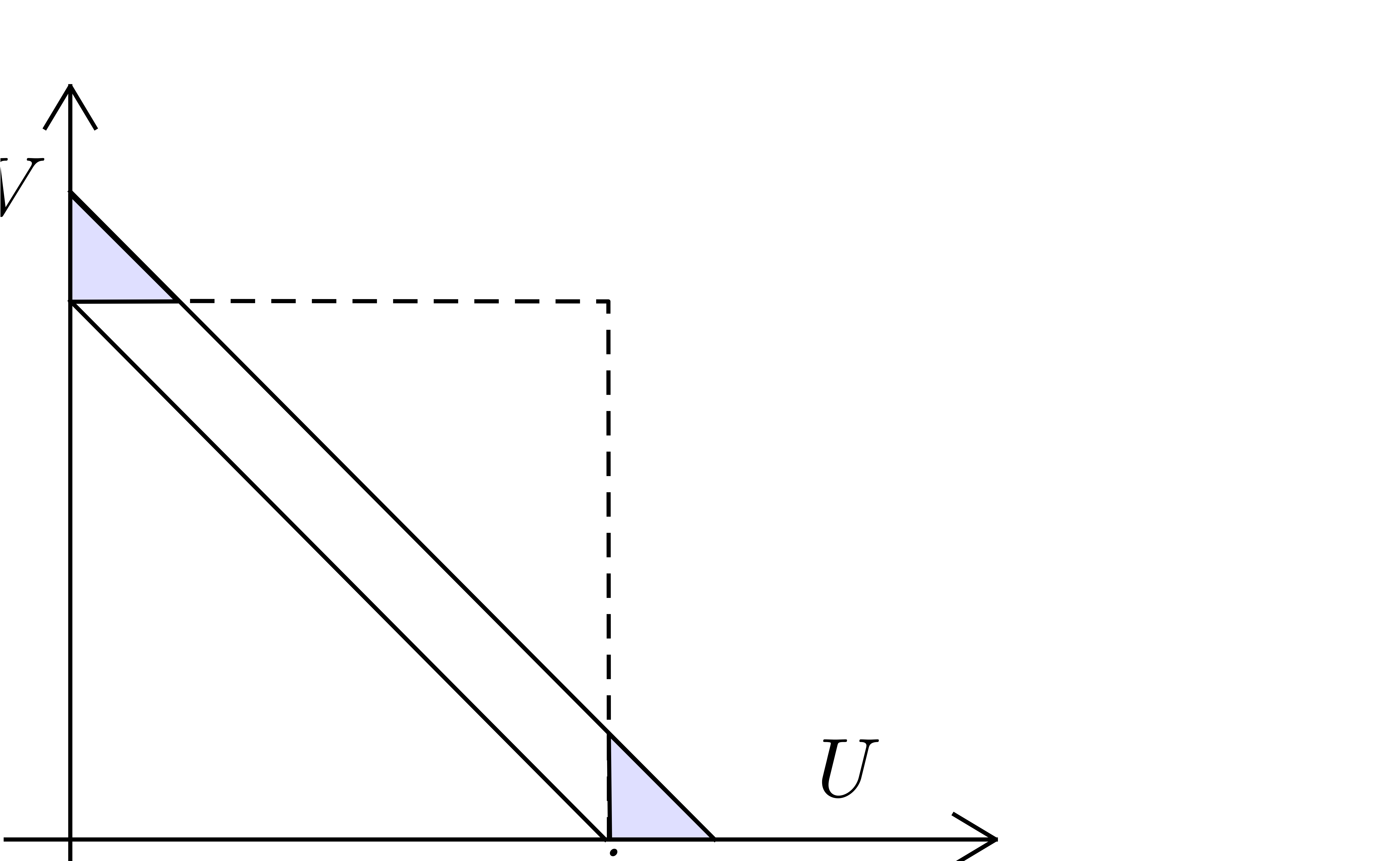
where  stands for the middle product (see figure
1). Instead of computing
stands for the middle product (see figure
1). Instead of computing  directly
using this formula, we will systematically work with the FFT transforms
directly
using this formula, we will systematically work with the FFT transforms
 of
of  at order
  and similarly for
  and
and  , so that

Recall that we may resort to TFT transforms [vdH04, vdH05] if is not a power of two. Now
assume that  ,
,  and
and

are known. Then the relation (10) yields
 |
(12) |
In practice, we compute  via
via  ,
,  and
and  , using FFT multiplication. Here we notice that
the FFT transforms of and
only need to be computed once.
, using FFT multiplication. Here we notice that
the FFT transforms of and
only need to be computed once.
Putting together what has been said and assuming that , and  are known, we have the following algorithm for the successive
computation of
are known, we have the following algorithm for the successive
computation of  :
:
for  do
do 
for  do
do


In this algorithm, the product is evaluated in a
lazy manner. Of course, using a straightforward adaptation, one may also
use a relaxed algorithm. In particular, the algorithm from [vdH03b]
is particularly well-suited in combination with middle products. In the
standard FFT model, [vdH03a] is even faster.
 has
has  non-zero
entries. Assume the standard FFT model. Then there exists an algorithm
which computes the truncated solution to
non-zero
entries. Assume the standard FFT model. Then there exists an algorithm
which computes the truncated solution to
 in time
  , provided that
 . In particular,
  .
.
Proof. In our algorithm, we take  , where
  grows very
slowly to infinity (such as
grows very
slowly to infinity (such as  ),
so that
),
so that  . Let us carefully
examine the cost of our algorithm for this choice of
. Let us carefully
examine the cost of our algorithm for this choice of  :
:
The computation of , and requires a time  .
.
The computation of the FFT-transforms  ,
,
 and the inverse transforms
  has the same complexity
  as the computation
of the final matrix product at order .
as the computation
of the final matrix product at order .
The computation of  middle products
  in the FFT-model requires a time
  . Using a relaxed multiplication algorithm,
the cost further reduces to
. Using a relaxed multiplication algorithm,
the cost further reduces to  .
.
The computation of the using the Newton
iteration (12) involves
Matrix FFT-transforms of and , of cost .
 vectorial FFT-transforms of cost
  .
.
 matrix vector multiplications in the
FFT-model, of cost
matrix vector multiplications in the
FFT-model, of cost  .
.
Adding up the different contributions completes the proof. Notice that
the computation of  more terms has negligible
cost, in the case when is not a multiple of
.
more terms has negligible
cost, in the case when is not a multiple of
.
Remark  ,
,  and
and  require an additional space overhead, when using
the polynomial adaptation [CK91, vdH02] of
Schönhage-Strassen multiplication. Consequently, the cost in point
require an additional space overhead, when using
the polynomial adaptation [CK91, vdH02] of
Schönhage-Strassen multiplication. Consequently, the cost in point
 now becomes

Provided that  , we obtain the
same complexity as in the theorem, by choosing
sufficiently slow.
, we obtain the
same complexity as in the theorem, by choosing
sufficiently slow.
Remark  with
(which corresponds to a fundamental system of solutions to (9)).
In that case, the complexity becomes
with
(which corresponds to a fundamental system of solutions to (9)).
In that case, the complexity becomes  .
.
Remark  denote the complexity of computing both and
 . One has

since the product  and the formulas (6)
and (7) give rise to
and the formulas (6)
and (7) give rise to  matrix
multiplications. This yields
matrix
multiplications. This yields  from which we may
subtract
from which we may
subtract  in the case when
  is not needed. The bound may be further improved to
  using [Sch00]. Similarly, the old bound for the resolution
of (9) is
using [Sch00]. Similarly, the old bound for the resolution
of (9) is  , or
, or
 when using [Sch00].
Remark  .
In practice, we may actually take
.
In practice, we may actually take  ,
in which case there is no particular penalty when using a naive
algorithm instead of a relaxed one. In fact, for larger values of
,
in which case there is no particular penalty when using a naive
algorithm instead of a relaxed one. In fact, for larger values of  , it is rather the hypothesis which is easily violated. In that case, one may take
 instead of
  and still
gain a constant factor between
and still
gain a constant factor between  and .
and .
Remark  of a power series
  . In that case, theorem 1 provides
a way to compute
. In that case, theorem 1 provides
a way to compute  in time
  , which yields an improvement over [Ber,
HZ]. Notice that FFT trading is a variant of Newton caching
in [Ber], but not exactly the same: in our case, we use an
“order ” Newton
iteration, whereas Bernstein uses classical Newton iterations on
block-decomposed series. In the case of power series division
, which yields an improvement over [Ber,
HZ]. Notice that FFT trading is a variant of Newton caching
in [Ber], but not exactly the same: in our case, we use an
“order ” Newton
iteration, whereas Bernstein uses classical Newton iterations on
block-decomposed series. In the case of power series division  at order or division with
remainder of a polynomial of degree
at order or division with
remainder of a polynomial of degree  by a
polynomial of degree
by a
polynomial of degree  , the
present technique also allows for improvements w.r.t. [Ber, HZ]. In both cases, the new complexity is
, the
present technique also allows for improvements w.r.t. [Ber, HZ]. In both cases, the new complexity is
 . In addition, we notice that
the technique of FFT trading allows for a “smooth junction”
between the Karatsuba (or Toom-Cook) model and the FFT model.
. In addition, we notice that
the technique of FFT trading allows for a “smooth junction”
between the Karatsuba (or Toom-Cook) model and the FFT model.
Assuming that one is able to solve the linearized version of an implicit equation (1), it is classical that Newton's method can again be used to solve the equation itself [BK78, vdH02, BCO+06]. Before we show how to do this for algebraic systems of differential equations, let us first give a few definitions for polynomial expressions.
Given a vector  of series variables, we will
represent polynomials in
of series variables, we will
represent polynomials in  by dags (directed
acyclic graphs), whose leaves are either series in
or variables , and whose
inner nodes are additions, subtractions or multiplications. An example
of such a dag is shown in figure 2. We will denote by
by dags (directed
acyclic graphs), whose leaves are either series in
or variables , and whose
inner nodes are additions, subtractions or multiplications. An example
of such a dag is shown in figure 2. We will denote by  and
and  the number of nodes which
occur as an operand resp. result of a multiplication. We
call
the number of nodes which
occur as an operand resp. result of a multiplication. We
call  the multiplicative size
  of the dag and the total number
  of
nodes the total size of the dag. Using the FFT, one may compute
of
nodes the total size of the dag. Using the FFT, one may compute
 in terms of in time
 .
.
 |
Now assume that we are given an -dimensional
system
 |
(13) |
with initial condition , and
where  is a tuple of
polynomials in
is a tuple of
polynomials in  . Given the
unique solution to this initial value problem,
consider the Jacobian matrix
. Given the
unique solution to this initial value problem,
consider the Jacobian matrix

Assuming that  is known, we may compute
  in time
  using automatic
differentiation. As usual, this complexity hides an
using automatic
differentiation. As usual, this complexity hides an  -dependent overhead, which is bounded by
  . For
. For  ,
we have
,
we have

so that
 |
(14) |
Let us again adopt the notation (11). Having determined
 and
and  for each
subexpression
for each
subexpression  of up to a
given order
of up to a
given order  , the computation
of and all
, the computation
of and all  can be done
in three steps:
can be done
in three steps:
The computation of all  ,
using lazy or relaxed evaluation, where
,
using lazy or relaxed evaluation, where  .
.
The determination of  using (14).
The computation of all .
We notice that and are
almost identical, since

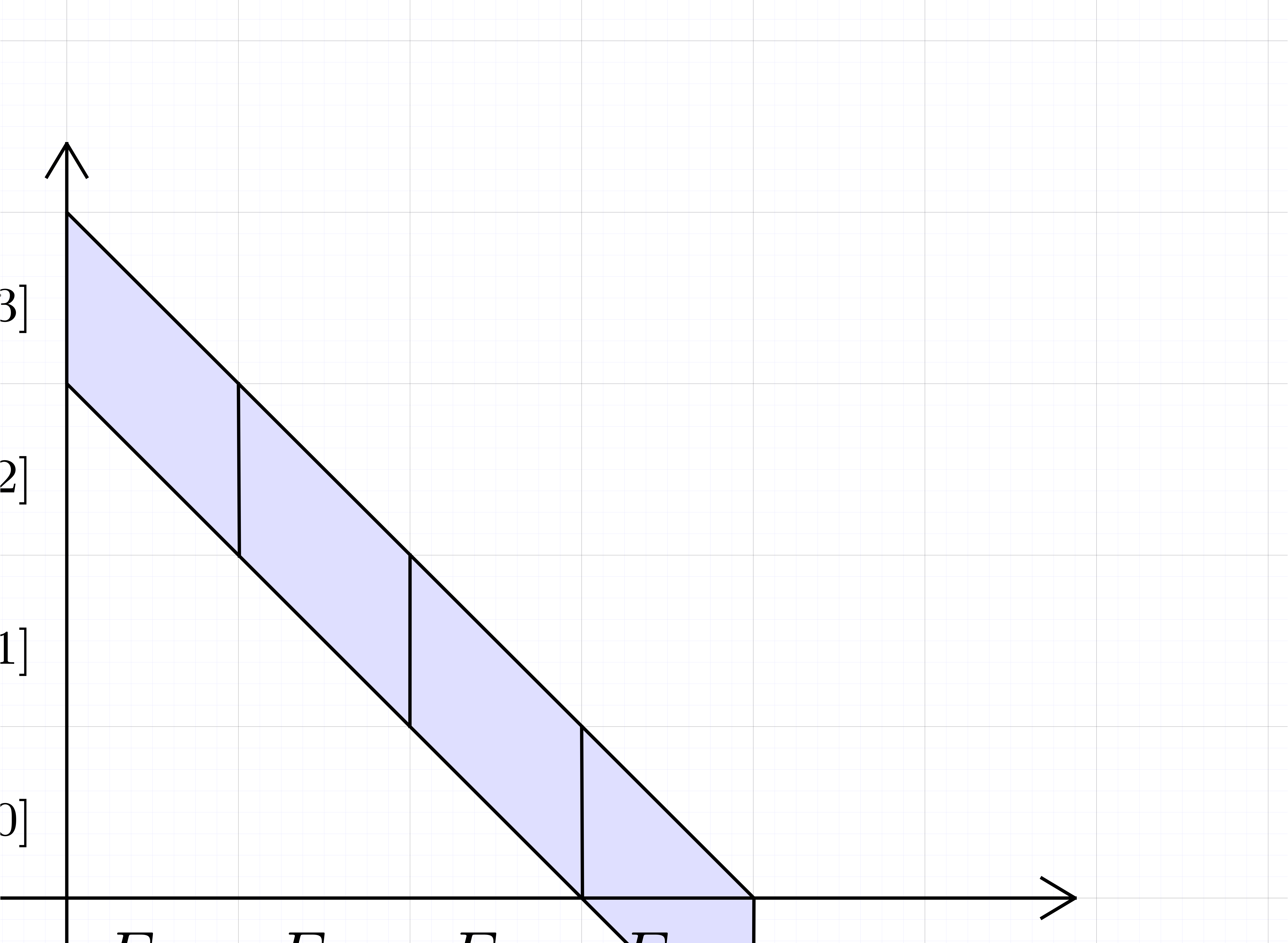
If  is a product, then
can be determined from
is a product, then
can be determined from  and
and  using a suitable middle product with “omitted extremes” (see
figure 3). Step 3 consists of an adjustment, which puts
these extremes back in the sum. Of course, the computations of products
can be done in a relaxed fashion.
using a suitable middle product with “omitted extremes” (see
figure 3). Step 3 consists of an adjustment, which puts
these extremes back in the sum. Of course, the computations of products
can be done in a relaxed fashion.
 |
-dimensional
system  is a polynomial, given by a dag of multiplicative size and total size
  .
Assume the standard FFT model. Then there exist an algorithm which
computes in time
.
Assume the standard FFT model. Then there exist an algorithm which
computes in time  ,
provided that .
,
provided that .
Proof. When working systematically with the
FFT-ed values of the , steps
and give rise to a cost
 for the FFT transforms and a cost
  for the scalar multiplications and additions. In a similar
way as in the proof of theorem 1, the computation of the
gives rise to a cost
for the scalar multiplications and additions. In a similar
way as in the proof of theorem 1, the computation of the
gives rise to a cost  . Again, the cost of the computation of the initial
and
. Again, the cost of the computation of the initial
and  is negligible.
Remark  in the synthetic FFT model and under the
assumption . This bound is
derived in a similar way as in remark 2.
in the synthetic FFT model and under the
assumption . This bound is
derived in a similar way as in remark 2.
Remark is not
entirely adequate for expressing the old complexity. In the worst case,
the old complexity is  , which
further improves to
, which
further improves to  using [Sch00].
However, the factor
using [Sch00].
However, the factor  is quite pessimistic, since
it occurs only when most of the subexpressions
of depend on most of the variables
is quite pessimistic, since
it occurs only when most of the subexpressions
of depend on most of the variables  . If the multiplicative subexpressions depend on an average number of
  variables
  , then the process
of automatic differentiation can be optimized so as to replace by in the bound (roughly
speaking).
, then the process
of automatic differentiation can be optimized so as to replace by in the bound (roughly
speaking).
It is well-known that discrete FFT transforms are most
efficient on blocks of size with . In particular, without taking particular
care, one may lose a factor  when computing the
product of two polynomials and
when computing the
product of two polynomials and  of degree
  with
with  .
One strategy to remove this problem is to use the TFT (truncated Fourier
transform) as detailed in [vdH04] with some corrections and
further improvements in [vdH05].
.
One strategy to remove this problem is to use the TFT (truncated Fourier
transform) as detailed in [vdH04] with some corrections and
further improvements in [vdH05].
An alternative approach is to cut and into  parts of size
  , where
  grows slowly to
infinity with . Let us denote
grows slowly to
infinity with . Let us denote

Attention to the minor change with respect to the notations from section
2. Now we multiply and by
FFT-ing the blocks and  at size .
Naively multiplying the resulting FFT-ed polynomials in  :
:

Transforming the result back.
This approach has a cost  which behaves more
“smoothly” as a function of .
which behaves more
“smoothly” as a function of .
In this particular case, it turns out that the TFT transform is always
better, because the additional linear factor  is
reduced to . However, in the
multivariate setting, the TFT also has its drawbacks. More precisely,
consider two multivariate polynomials
is
reduced to . However, in the
multivariate setting, the TFT also has its drawbacks. More precisely,
consider two multivariate polynomials  whose
supports have a “dense flavour”. Typically, we may assume
the supports to be convex subsets of
whose
supports have a “dense flavour”. Typically, we may assume
the supports to be convex subsets of  .
In addition one may consider truncated products, where we are only
interested in certain monomials of the product. In order to apply the
TFT, one typically has to require in addition that the supports of and are initial segments of
. Even then, the overhead for
certain types of supports may increase if
.
In addition one may consider truncated products, where we are only
interested in certain monomials of the product. In order to apply the
TFT, one typically has to require in addition that the supports of and are initial segments of
. Even then, the overhead for
certain types of supports may increase if  gets
large.
gets
large.
One particularly interesting case for complexity studies is the
computation of the truncated product of two dense polynomials and with total degree . This is typically encountered in the
integration of dynamical systems using Taylor models. Although the TFT
is a powerful tool for small dimensions  ,
FFT trading might be an interesting complement for moderate dimensions
,
FFT trading might be an interesting complement for moderate dimensions
 . For really huge dimensions,
one may use [LS03] or [vdH02, Section 6.3.5].
The idea is again to cut in blocks
. For really huge dimensions,
one may use [LS03] or [vdH02, Section 6.3.5].
The idea is again to cut in blocks

where is small (and
preferably a power of two). Each block is then transformed using a
suitable TFT transform (notice that the supports of the blocks are still
initial segments when restricted to the block). We next compute the
truncated product of the TFT-ed polynomials  and
and
 in a naive way and TFT back. The naive
multiplication step involves
in a naive way and TFT back. The naive
multiplication step involves

multiplications of TFT-ed blocks. We may therefore hope for some gain
whenever  is small with respect to
  . We always gain for
  and usually also for
  , in
which case
, in
which case  . Even for
  , when
  , it is quite possible that one may gain in
practice.
, it is quite possible that one may gain in
practice.
The main advantage of the above method over other techniques, such as
the TFT, is that the shape of the support is preserved during the
reduction  (as well as for the “destination
support”). However, the TFT also allows for some additional tricks
[vdH05, Section 9] and it is not yet clear to us which
approach is best in practice. Of course, the above technique becomes
even more useful in the case of more general truncated multiplications
for dense supports with shapes which do not allow for TFT
multiplication.
(as well as for the “destination
support”). However, the TFT also allows for some additional tricks
[vdH05, Section 9] and it is not yet clear to us which
approach is best in practice. Of course, the above technique becomes
even more useful in the case of more general truncated multiplications
for dense supports with shapes which do not allow for TFT
multiplication.
For small values of , we
notice that the pair/odd version of Karatsuba multiplication presents
the same advantage of geometry preservation (see [HZ02] for
the one-dimensional case). In fact, fast multiplication using FFT
trading is quite analogous to this method, which generalizes for
Toom-Cook multiplication. In the context of numerical computations, the
property of geometry preservation is reflected by increased numerical
stability.
To finish, we would like to draw the attention of the reader to another
advantage of FFT trading: for really huge values of , it allows for the reduction of the memory
consumption. For instance, assume that we want to multiply two truncated
power series and at
order . With the above
notations, one may first compute  .
For
.
For  , we next compute
  ,
,  and
and  . The idea is now that
  are no longer used at stage ,
so we may remove them from memory.
are no longer used at stage ,
so we may remove them from memory.
We have summarized the main results of this paper in tables 1
and 2. We recall that in the
standard FFT model and otherwise. In practice,
we expect that the factor behaves very much like
a constant, which equals  at the point where we
enter the FFT model. Consequently, we expect the new algorithms to
become only interesting for quite large values of . We plan to come back to this issue as soon as
implementations of all algorithms will be available in the
at the point where we
enter the FFT model. Consequently, we expect the new algorithms to
become only interesting for quite large values of . We plan to come back to this issue as soon as
implementations of all algorithms will be available in the  .
.
|
||||||||||
A final interesting question is to which extent Newton's method can be generalized. Clearly, it is not hard to consider more general equations of the kind

since the series  merely act as perturbations.
However, it seems harder (but maybe not impossible) to deal with
equations of the type
merely act as perturbations.
However, it seems harder (but maybe not impossible) to deal with
equations of the type

since it is not clear a priori how to generalize the concept of
a fundamental system of solutions and its use in the Newton iteration.
In the case of partial differential equations with initial conditions on
a hyperplane, the fundamental system of solutions generally has infinite
dimension, so essentially new ideas would be needed here. Nevertheless,
the strategy of relaxed evaluation applies in all these cases, with the
usual overhead in general and
overhead in the synthetic FFT model.
A. Bostan, F. Chyzak, F. Ollivier, B. Salvy, É. Schost, and A. Sedoglavic. Fast computation of power series solutions of systems of differential equation. preprint, april 2006. submitted, 13 pages.
D. Bernstein. Removing redundancy in high precision Newton iteration. Available from http://cr.yp.to/fastnewton.html.
R.P. Brent and H.T. Kung. Fast algorithms for manipulating formal power series. Journal of the ACM, 25:581–595, 1978.
D.G. Cantor and E. Kaltofen. On fast multiplication of polynomials over arbitrary algebras. Acta Informatica, 28:693–701, 1991.
S.A. Cook. On the minimum computation time of functions. PhD thesis, Harvard University, 1966.
J.W. Cooley and J.W. Tukey. An algorithm for the machine calculation of complex Fourier series. Math. Computat., 19:297–301, 1965.
Guillaume Hanrot, Michel Quercia, and Paul Zimmermann. The middle product algorithm I. speeding up the division and square root of power series. AAECC, 14(6):415–438, 2004.
G. Hanrot and P. Zimmermann. Newton iteration revisited. http://www.loria.fr/ zimmerma/papers/fastnewton.ps.gz.
Guillaume Hanrot and Paul Zimmermann. A long note on Mulders' short product. Research Report 4654, INRIA, December 2002. Available from http://www.loria.fr/ hanrot/Papers/mulders.ps.
A. Karatsuba and J. Ofman. Multiplication of multidigit numbers on automata. Soviet Physics Doklady, 7:595–596, 1963.
R. Lohner. Einschließung der Lösung gewöhnlicher Anfangs- und Randwertaufgaben und Anwendugen. PhD thesis, Universität Karlsruhe, 1988.
R. Lohner. On the ubiquity of the wrapping effect in the computation of error bounds. In U. Kulisch, R. Lohner, and A. Facius, editors, Perspectives of enclosure methods, pages 201–217. Springer, 2001.
G. Lecerf and É. Schost. Fast multivariate power series multiplication in characteristic zero. SADIO Electronic Journal on Informatics and Operations Research, 5(1):1–10, September 2003.
K. Makino and M. Berz. Remainder differential algebras and their applications. In M. Berz, C. Bischof, G. Corliss, and A. Griewank, editors, Computational differentiation: techniques, applications and tools, pages 63–74, SIAM, Philadelphia, 1996.
K. Makino and M. Berz. Suppression of the wrapping effect by taylor model-based validated integrators. Technical Report MSU Report MSUHEP 40910, Michigan State University, 2004.
R.T. Moenck and J.H. Carter. Approximate algorithms to derive exact solutions to systems of linear equations. In Symbolic and algebraic computation (EUROSAM '79, Marseille), volume 72 of LNCS, pages 65–73, Berlin, 1979. Springer.
R.E. Moore. Interval analysis. Prentice Hall, Englewood Cliffs, N.J., 1966.
V. Pan. How to multiply matrices faster, volume 179 of Lect. Notes in Math. Springer, 1984.
G. Schulz. Iterative Berechnung der reziproken Matrix. Z. Angew. Math. Mech., 13:57–59, 1933.
A. Schönhage. Variations on computing reciprocals of power series. Inform. Process. Lett., 74:41–46, 2000.
A. Schönhage and V. Strassen. Schnelle Multiplikation grosser Zahlen. Computing 7, 7:281–292, 1971.
V. Strassen. Gaussian elimination is not optimal. Numer. Math., 13:352–356, 1969.
A.L. Toom. The complexity of a scheme of functional elements realizing the multiplication of integers. Soviet Mathematics, 4(2):714–716, 1963.
J. van der Hoeven. Lazy multiplication of formal power series. In W. W. Küchlin, editor, Proc. ISSAC '97, pages 17–20, Maui, Hawaii, July 1997.
J. van der Hoeven. Relax, but don't be too lazy. JSC, 34:479–542, 2002.
J. van der Hoeven. New algorithms for relaxed multiplication. Technical Report 2003-44, Université Paris-Sud, Orsay, France, 2003.
J. van der Hoeven. Relaxed multiplication using the middle product. In Manuel Bronstein, editor, Proc. ISSAC '03, pages 143–147, Philadelphia, USA, August 2003.
J. van der Hoeven. The truncated Fourier transform and applications. In J. Gutierrez, editor, Proc. ISSAC 2004, pages 290–296, Univ. of Cantabria, Santander, Spain, July 4–7 2004.
J. van der Hoeven. Notes on the Truncated Fourier Transform. Technical Report 2005-5, Université Paris-Sud, Orsay, France, 2005.
J. van der Hoeven. On effective analytic continuation. Technical Report 2006-15, Univ. Paris-Sud, 2006.
J. van der Hoeven et al. Mmxlib: the standard library for Mathemagix, 2002–2006. http://www.mathemagix.org/mml.html.
Winograd and Coppersmith. Matrix multiplication via
arithmetic progressions. In Proc. of the  Annual Symposium on Theory of Computing, pages 1–6,
New York City, may 25–27 1987.
Annual Symposium on Theory of Computing, pages 1–6,
New York City, may 25–27 1987.
 .
. denotes the complexity in order two polynomials of
degree
denotes the complexity in order two polynomials of
degree  and trading the remaining Newton steps against a lazy or relaxed
algorithm in a suitable FFT model.
and trading the remaining Newton steps against a lazy or relaxed
algorithm in a suitable FFT model.


 using middle products.
 ,
, (since
  and
and  )and
)and .
. in the multiplicative size.
 .
. .
.


 of linear differential equations
up to
of linear differential equations
up to  ).
).


 up to
up to  ,
,