|
|
A. Laboratoire d'informatique de l'École polytechnique, LIX, UMR 7161 CNRS, Bâtiment Alan Turing, CS35003, 1, rue Honoré d'Estienne d'Orves, 91120 Palaiseau, France, vdhoeven@lix.polytechnique.fr
B. Laboratoire d'informatique de l'École polytechnique, LIX, UMR 7161 CNRS, Bâtiment Alan Turing, CS35003, 1, rue Honoré d'Estienne d'Orves, 91120 Palaiseau, France, marc@mezzarobba.net
 . This work has
been supported by an ERC-2023-ADG grant for the ODELIX project
(number 101142171).
. This work has
been supported by an ERC-2023-ADG grant for the ODELIX project
(number 101142171).
Funded by the European Union. Views and opinions expressed are however those of the author(s) only and do not necessarily reflect those of the European Union or the European Research Council Executive Agency. Neither the European Union nor the granting authority can be held responsible for them. |
 |
 . This article has
been written using GNU TeXmacs [37].
. This article has
been written using GNU TeXmacs [37].
In this paper we study hardware-accelerated integer matrix multiplication, with coefficients of sizes between 8 and 1000 bits. More particularly, we study two relatively new hardware features in Intel CPUs: the IFMA “integer FMA” instruction and the AMX matrix extensions. We study various algorithms and analyze to what extent our implementations on top of the JIL library can approach theoretical peak performance.
Arguably the most significant recent trend in computer hardware is the eruption of tensor cores in both GPUs and CPUs. Although driven by applications in artificial intelligence, is there a potential for tensor cores to be used for other purposes? After all, GPUs have found many applications beyond their initial ones in the gaming industry.
The main motivation of this paper is to study this question for
applications in scientific computation and more particularly in computer
algebra and computer arithmetic. We will focus on the problem of  matrix multiplication with
  -bit integer entries. Tensor cores are designed to
accelerate such computations in the case where
-bit integer entries. Tensor cores are designed to
accelerate such computations in the case where  is large and
  . Can this be
used to efficiently deal with other bit precisions, ranging from small
ones like
. Can this be
used to efficiently deal with other bit precisions, ranging from small
ones like  to larger ones like
  ?
?
We mainly restrict our attention to the multiplication of square matrices. This is indeed most favorable for tensor
cores, but also most significant from a complexity perspective, since
the complexity of many problems in linear algebra and beyond can be
expressed in terms of the complexity of square matrix products [5].
Of course, this restriction will also simplify comparisons, because
varying both and will
already give rise to numerous different cases, as we shall see.
To be fair, we should also compare implementations that exploit tensor
cores with alternative ones that are based on more conventional vector
arithmetic. For this reason, we chose to focus on recent  matrix FMA (MFMA)
  in about
  cycles, where
  and
and  (of dimensions
  and
and
 ) have
  -bit entries and
  (of
dimension
(of
dimension  ) has 32-bit
entries. Roughly speaking, an integer FMA (IFMA) allow us to compute
) has 32-bit
entries. Roughly speaking, an integer FMA (IFMA) allow us to compute
 in one cycle, where
  and
and
 are -wide
vectors of
are -wide
vectors of  -bit integers and
 is an -wide
vector of
is an -wide
vector of  -bit integers. Note
that we preferred the terminology MFMA over GeMM and (general matrix
multiplication
-bit integers. Note
that we preferred the terminology MFMA over GeMM and (general matrix
multiplication  ) because AMX
only supports positive accumulation.
) because AMX
only supports positive accumulation.
In this paper, we focus on the performance of implementations that use a single core of our CPU. This simplification allows to measure the relevance of different implementation strategies that exploit different hardware features (IFMA or AMX), without being distracted by mostly orthogonal considerations on how to scale up these base implementations on multi-core architectures.
All our timings will be relative to theoretical peak performance. For
instance, for a naive implementation of matrix
multiplication using  IFMAs, we will report on
the cost of the matrix multiplication divided by the theoretical cost to
perform IFMAs. These ratios are fairly
independent of the particular machine on which we execute our programs
and indicate the quality of our implementation. Quotients close to one
mean that we could not have done much better for the algorithm at hand.
Higher ratios indicate potential problems such as suboptimal memory
access patterns or asymptotically subdominant costs that become high for
certain sizes. In an ideal world in which all ratios are one, the
theoretical complexity analysis of our methods would correspond
perfectly to their practical performance. For completeness, we also
added an appendix with absolute timings, both for our new implementation
and some existing software.
IFMAs, we will report on
the cost of the matrix multiplication divided by the theoretical cost to
perform IFMAs. These ratios are fairly
independent of the particular machine on which we execute our programs
and indicate the quality of our implementation. Quotients close to one
mean that we could not have done much better for the algorithm at hand.
Higher ratios indicate potential problems such as suboptimal memory
access patterns or asymptotically subdominant costs that become high for
certain sizes. In an ideal world in which all ratios are one, the
theoretical complexity analysis of our methods would correspond
perfectly to their practical performance. For completeness, we also
added an appendix with absolute timings, both for our new implementation
and some existing software.
All implementations in this paper are done inside or on top of the C++ library JIL [2, 40] for computations with straight-line programs (SLPs). This work is the first step of a project to the JIL library with fast linear algebra over the integers and fixed point numbers. We would like to cover all ranges of matrix dimensions and bit-sizes of the integers, while taking advantage of recent hardware features such as IFMA and AMX.
Conversely, matrix multiplication is an excellent problem for extending JIL beyond the mere compilation of SLPs. Another important motivation behind the present work is to use matrix multiplication as a case study for how to integrate SLPs inside larger pieces of code such as multiple loops. The integration of AMX instructions into the SLP framework is also a challenge.
Multiple precision integer multiplication has a long history and there exist many algorithms for various bit precisions, such as the traditional schoolbook method, Karatsuba's algorithm [43], Toom's method [62], and modular methods [24, Chapter 5]. For high precisions, there are also methods based on the fast Fourier transform [11, 57, 34], but we will not use them in this paper. GMP [28] and MPFR [31] are the reference libraries for multiple precision integer and floating point arithmetic. We also refer to [38, 29, 18, 8, 39] for some recent work on this topic in the HPC context.
In the context of integer matrix multiplication, fast multiple precision
methods tend to become useful at already very low precisions. This is
due to the fact that all known methods can be regarded as
modular or evaluation-interpolation methods. Roughly
speaking, multiplying two matrices with  -bit entries is reduced to
  multiplications of matrices
with -bit entries, where the
quantity depends on the method (this will be
detailed in Section 3 and Table 1 below). The
cost of this reduction scales with
multiplications of matrices
with -bit entries, where the
quantity depends on the method (this will be
detailed in Section 3 and Table 1 below). The
cost of this reduction scales with  ,
whereas the cost of the low precision matrix
multiplications scales with
,
whereas the cost of the low precision matrix
multiplications scales with  .
Consequently, the cost of the reduction becomes negligible for large
and, for a given
.
Consequently, the cost of the reduction becomes negligible for large
and, for a given  ,
it is recommended to pick the method for which
is minimal. Good practical implementations should reflect this fact and
this is indeed what our work aims at.
,
it is recommended to pick the method for which
is minimal. Good practical implementations should reflect this fact and
this is indeed what our work aims at.
Theoretically speaking [67],
matrices can be multiplied in time  with
with  for large .
However, among the asymptotically faster algorithms with
for large .
However, among the asymptotically faster algorithms with  , only Strassen's algorithm [60]
with
, only Strassen's algorithm [60]
with  has allowed for some modest practical gains
so far. The recent trend to accelerate matrix multiplication directly in
the hardware leads to more significant practical gains. (In fact, these
hardware accelerations make the practical complexity of matrix
multiplication behave as if
has allowed for some modest practical gains
so far. The recent trend to accelerate matrix multiplication directly in
the hardware leads to more significant practical gains. (In fact, these
hardware accelerations make the practical complexity of matrix
multiplication behave as if  were well below
 . The potential impact of
this observation is another motivation behind our work.)
. The potential impact of
this observation is another motivation behind our work.)
Several works [12, 19] and research
implementations [50, 49] specifically address
the challenges raised by Intel's AMX technologies.
Before the emergence of tensor cores, classical reference
implementations for matrix multiplication and other routines from linear
algebra include
Our work on JIL also draws inspiration from the compilation of codelets
for critical tasks as pioneered in
We report on an experimental HPC implementation of integer matrix
multiplication for a wide range of matrix dimensions and bit sizes of
integers. We have spent a comparable amount of effort on exploiting two
types of hardware acceleration, namely the IFMA and AMX extensions in
recent Intel processors. In Table 1, we presented an
idealized complexity model for large matrix dimensions as a function of
the bit size of the coefficients and the integer multiplication method
being used. Although the underlying methods are not new, we expect this
synthesis to be useful as a guideline for implementors. Our
implementations indeed often come close to the theoretical peak
performance for which our idealized model is most relevant. This holds
especially for our IFMA-based implementation and a bit less for the
AMX-based one. For “large” matrices,
say  , we observe that
AMX-based algorithms outperform the IFMA-based ones. Although the gain
is modest for now, we expect that it can be improved with more work.
Another potential advantage of AMX is that we have a more fine-grained
control over the bit-precision. Our implementations also outperform the
current reference libraries
, we observe that
AMX-based algorithms outperform the IFMA-based ones. Although the gain
is modest for now, we expect that it can be improved with more work.
Another potential advantage of AMX is that we have a more fine-grained
control over the bit-precision. Our implementations also outperform the
current reference libraries
Throughout this paper, we will write  for the set
of positive integers, including zero, and
for the set
of positive integers, including zero, and  for
the set of unsigned -bit
integers.
for
the set of unsigned -bit
integers.
Given a ring  and
and  ,
we write
,
we write  for the set of vectors
  of length with entries in . We will also write
  for the
set of polynomials of degree
for the
set of polynomials of degree  in
over . We will assume the
natural dense representation for such polynomials
in
over . We will assume the
natural dense representation for such polynomials  by their vectors of coefficients.
We formally extend the polynomial notation to the case when is replaced by an integer radix , typically of the form  for
some
for
some  . This allows us to
rewrite unsigned integers in
. This allows us to
rewrite unsigned integers in  as
“polynomials”
as
“polynomials”  in the radix.
Following terminology from GMP [28], it is customary to
call the coefficients
in the radix.
Following terminology from GMP [28], it is customary to
call the coefficients  limbs. If
  is a machine integer type, then we may represent an
integer by its vector
is a machine integer type, then we may represent an
integer by its vector  of
limbs.
of
limbs.
For dimensions  , we also
write
, we also
write  for the set of
  matrices with entries in .
Unless stated otherwise, we will always assume that matrices
matrices with entries in .
Unless stated otherwise, we will always assume that matrices  are represented in row-major order on a computer, as
vectors
are represented in row-major order on a computer, as
vectors  . By “
 matrix multiplication”, we understand the
multiplication of an
matrix multiplication”, we understand the
multiplication of an  matrix with an
  matrix into an matrix.
Let  be the machine precision (or one of the
available machine precisions). Standard arithmetic operations on naturally extend to SIMD vectors of width
be the machine precision (or one of the
available machine precisions). Standard arithmetic operations on naturally extend to SIMD vectors of width  in
in  . Whenever a
function that only involves basic arithmetic operations needs to be
evaluated exactly times, this can be done
replacing all operations by their SIMD versions.
. Whenever a
function that only involves basic arithmetic operations needs to be
evaluated exactly times, this can be done
replacing all operations by their SIMD versions.
For instance, given a matrix  and a vector
  , consider the function that
computes the matrix-vector product
, consider the function that
computes the matrix-vector product  .
If we need to evaluate this function times, then
the simplest solution is to present the input as a matrix
.
If we need to evaluate this function times, then
the simplest solution is to present the input as a matrix  and a vector
  ,
in which case the exact same formula
,
in which case the exact same formula  yields all
matrix-vector products in SIMD format.
yields all
matrix-vector products in SIMD format.
We call this way of vectorizing the pure SIMD mode. This works
best whenever a given function needs to be evaluated a multiple of times. This also assumes that all data types are
replaced functorially by their standard vectorized versions.
For instance, the standard vectorization of the matrix type  is
is  . The
standard vectorization of a multiple precision integer type
. The
standard vectorization of a multiple precision integer type  consists of working with “limbs” that are
vectors in . Hence SIMD
multiple precision integers
consists of working with “limbs” that are
vectors in . Hence SIMD
multiple precision integers  are represented as
 with
with  and . Note that this may not seem to be most
“natural”, since one might prefer to represent as
and . Note that this may not seem to be most
“natural”, since one might prefer to represent as  with
with  .
.
SIMD arithmetic can often be used as well for evaluating a function only
once. For instance, the multiplication  of two
matrices
of two
matrices  and
and  can benefit
from SIMD acceleration whenever
can benefit
from SIMD acceleration whenever  is a multiple of
the SIMD width . Indeed, it
suffices to reinterpret as a matrix
is a multiple of
the SIMD width . Indeed, it
suffices to reinterpret as a matrix  and as a matrix
  , while casting to a
matrix
, while casting to a
matrix  by repeating each of its entries times. After that, we can compute
  in the pure SIMD mode. However, these reinterpretations require some
gymnastics at least, and exploiting SIMD arithmetic becomes even more
delicate when none of the dimensions
in the pure SIMD mode. However, these reinterpretations require some
gymnastics at least, and exploiting SIMD arithmetic becomes even more
delicate when none of the dimensions  are a
multiple of . We will come
back to this tinkered SIMD mode in Section 4.3
below.
are a
multiple of . We will come
back to this tinkered SIMD mode in Section 4.3
below.
In this paper, we mainly report on relative timings with respect to the
theoretical peak performance. The only exception is the appendix, which
contains absolute timings, as well as timings for existing software. All
benchmarks were obtained on an
Let be our favorite (and supported) machine bit
precision for integer arithmetic, like  or
or  . The standard machine
representation of an integer
. The standard machine
representation of an integer  is the vector
  of “its” limbs.
The hardware is assumed to provide an instruction for multiplying two
limbs  , with a result in
  (sometimes, the low and high parts need to be
computed separately). For small precisions, multiple precision libraries
typically implement integer multiplications
(sometimes, the low and high parts need to be
computed separately). For small precisions, multiple precision libraries
typically implement integer multiplications  by
cross multiplying all limbs
by
cross multiplying all limbs  and summing the
results while handling carries appropriately.
and summing the
results while handling carries appropriately.
Unfortunately, carry propagation is unpleasant to vectorize and SIMD
units typically do not provide “vector carry registers”
(except for certain GPUs that handle this via mask registers). In a SIMD
world, it is therefore more convenient to work with redundant
representations: we still represent integers as polynomials  in some radix
  ,
but the limbs
,
but the limbs  are stored with a higher precision
 (which may be different for multiplicands and
products). If
(which may be different for multiplicands and
products). If  , then
  and the representation is said to be
normalized. We will call the bit
precision and the bit capacity.
The difference
and the representation is said to be
normalized. We will call the bit
precision and the bit capacity.
The difference  is the number nail bits
in the terminology of GMP.
is the number nail bits
in the terminology of GMP.
On recent Intel Xeon processors there are two instructions  and
and  for integer FMAs
(IFMA). Formally, given
for integer FMAs
(IFMA). Formally, given  and
and  , we have

where  and
and  denote the
quotient and the remainder of the euclidean division of
denote the
quotient and the remainder of the euclidean division of  by
by  . The IFMA
representation is the redundant representation with
. The IFMA
representation is the redundant representation with  and
and  . Given a
two-limb integer
. Given a
two-limb integer  , we can
accumulate
, we can
accumulate  the product of two limbs using one and one . As long as
  ,
this computation does not overflow, but
,
this computation does not overflow, but  typically does not remain normalized.
On even more recent Intel Xeon processors with AMX support, there is an
instruction for matricial FMAs  ,
where
,
where  ,
,  , and
, and  .
For individual integer coefficients of the product, this corresponds to
working with a redundant AMX representation with
.
For individual integer coefficients of the product, this corresponds to
working with a redundant AMX representation with  and
and  . Note that
products of limbs are two limbs long for the IFMA representation, but
only one limb long for the AMX representation. Indeed, when using AMX,
products and multiplicands are represented using limbs of different
. Note that
products of limbs are two limbs long for the IFMA representation, but
only one limb long for the AMX representation. Indeed, when using AMX,
products and multiplicands are represented using limbs of different
 -bit and -bit capacities, respectively.
Redundant representations have the advantage that the
nail bits can be used to accumulate carries, while postponing
normalization to the very end.
Consider for instance the multiplication of  and
and
 using integer FMAs, where
  and
and  . Assume also that
  . Then we first compute the
non-normalized product
. Then we first compute the
non-normalized product  with
with  , and then normalize it, as follows:

This algorithm has been represented graphically in Figure 1;
the lower and upper triangles correspond to and
operations, respectively.
If  , then the mere highest
limbs of the result can be computed similarly.
With the naive algorithm, the right picture in Figure 1
shows that this can be done at roughly half the cost of a full
multiplication. This is very useful for fixed point arithmetic, by
representing unsigned -limb
fixed point numbers as -limb
integers divided by
, then the mere highest
limbs of the result can be computed similarly.
With the naive algorithm, the right picture in Figure 1
shows that this can be done at roughly half the cost of a full
multiplication. This is very useful for fixed point arithmetic, by
representing unsigned -limb
fixed point numbers as -limb
integers divided by  . It is
interesting to note that the nail bits can be
exploited to represent small integer parts in this case.
. It is
interesting to note that the nail bits can be
exploited to represent small integer parts in this case.
However, our current implementation is limited to unsigned fixed point
numbers. Signed variants can be obtained by representing signed integers
 by
by
 and
and
 in
in
 ,
so that
,
so that
 .
Alternatively, one may use a two-complement representation for the
highest limb and adapt multiple precision multiplication accordingly.
But it becomes harder to exploit the extra
nail bits in both cases.
.
Alternatively, one may use a two-complement representation for the
highest limb and adapt multiple precision multiplication accordingly.
But it becomes harder to exploit the extra
nail bits in both cases.
We briefly discussed pure SIMD vectorization of multiple precision
integers in Section 2.2. The idea to represent such
integers as polynomials in  with vectorial limbs
also works for redundant representations. This allows us to apply the
algorithms from the previous subsection directly to pure SIMD multiple
precision integers in
with vectorial limbs
also works for redundant representations. This allows us to apply the
algorithms from the previous subsection directly to pure SIMD multiple
precision integers in  .
.
In a similar way, matrices of multiple precision integers in  can be rewritten into polynomials in
  with matrix limbs in
  .
Computing a non-normalized product
.
Computing a non-normalized product  with
with  ,
,  ,
and
,
and  can then be done naively using
  AMX-accelerated matrix multiplications
  . Note that we do not compute low and high
parts separately in this case. When doing high -limb multiplication in this way, this means that we
need to do
. Note that we do not compute low and high
parts separately in this case. When doing high -limb multiplication in this way, this means that we
need to do  multiplications, which is slightly
more than one half of the number for full products.
multiplications, which is slightly
more than one half of the number for full products.
For large matrix multiplications with -limb coefficients, using a naive
algorithm for polynomial multiplication becomes suboptimal. If  is small, then it becomes better to use Karatsuba's
algorithm [43].
is small, then it becomes better to use Karatsuba's
algorithm [43].
Given a ring , the
traditional Karatsuba trick reduces one multiplication  with
with  into three multiplications in and several additions and subtractions using the formulas
 ,
,  , and
, and  .
This trick generalizes to the case where is
replaced by
.
This trick generalizes to the case where is
replaced by  and by
  , in which case the multiplication
of two polynomials
, in which case the multiplication
of two polynomials  essentially reduces to three
multiplications of polynomials in .
These latter polynomials can be computed recursively using the same
trick.
essentially reduces to three
multiplications of polynomials in .
These latter polynomials can be computed recursively using the same
trick.
When working with multiple precision integers  one technical difficulty is that
  and
and  are in
  and not necessarily in
. This makes it better to
work with limbs of bit-size
and not necessarily in
. This makes it better to
work with limbs of bit-size  instead of . If our input integers used -bit limbs, then this requires them
to be rewritten into the
instead of . If our input integers used -bit limbs, then this requires them
to be rewritten into the  -bit
limb representation and vice versa for the output. When using
Karatsuba's algorithm recursively for
-bit
limb representation and vice versa for the output. When using
Karatsuba's algorithm recursively for  -limb
integers, we may either directly use limbs of bit-size
-limb
integers, we may either directly use limbs of bit-size  (which yields a multiplication algorithm for
  -bit integers), or do the limb rewritings
recursively as well (which yields a multiplication algorithm for
-bit integers), or do the limb rewritings
recursively as well (which yields a multiplication algorithm for  -bit integers).
Karatsuba's trick can also be applied to matrices  . In that case, we need to do
  multiplications in , but only
 additions and subtractions, which becomes
negligible for large .
Asymptotically, we thus gain a factor
additions and subtractions, which becomes
negligible for large .
Asymptotically, we thus gain a factor  with
respect to naive integer matrix multiplication.
with
respect to naive integer matrix multiplication.
Toom generalized Karatsuba's trick [62] and gave a way to
reduce the multiplication of two polynomials in
to  multiplications in at
the cost of an increased loss of bit-precision for the integer variant.
Interestingly, Karatsuba's trick can also be used directly for
multiplications in at
the cost of an increased loss of bit-precision for the integer variant.
Interestingly, Karatsuba's trick can also be used directly for  , while losing a single bit of
precision.
, while losing a single bit of
precision.
The idea (see also [36, Section 4.4.1], [44],
[9, Exercise 1.4], and [58]) is to observe
that the contribution of  to
to  can be computed using
  , for
all
, for
all  . In this way, we need to
first compute the products
. In this way, we need to
first compute the products  and then
  further products of the form
  , which yields a total number of
products. If we just want the high coefficients
, which yields a total number of
products. If we just want the high coefficients
 , then we only need to do
 multiplications. This is actually just as good
as Toom's algorithm for
multiplications. This is actually just as good
as Toom's algorithm for  and almost as good for
 and
and  .
.
A well known method for multiplying two matrices  is based on the Chinese remainder theorem. We first pick
  pairwise coprime moduli
  .
Best is to choose them as large as possible while fitting into bits. Let
.
Best is to choose them as large as possible while fitting into bits. Let  and assume that
  for some small
  with
with  .
.
In order to compute  , we
first reduce and modulo
, we
first reduce and modulo
 for
for  .
There is an elegant way to evaluate the map
.
There is an elegant way to evaluate the map  using a vector-matrix product [13]:

Taking the limbs of the entries of as our rows
, the computation of  for
for  thus essentially reduces
to an
thus essentially reduces
to an  matrix product over
and similarly for . We next
compute
matrix product over
and similarly for . We next
compute

for . We finally recover from  by applying the Chinese
remainder theorem. Consider the map
by applying the Chinese
remainder theorem. Consider the map  with
with  and
and  for . We have

where  is the inverse of
  modulo for .
After precomputing the -adic
expansions
modulo for .
After precomputing the -adic
expansions  , it is again
possible to compute
, it is again
possible to compute  using a vector-matrix
product [13]:
using a vector-matrix
product [13]:
In a similar way as above, the recovery of from
thus essentially boils down to an  matrix product over .
In order to ease the computation of the remainder with respect to
matrix product over .
In order to ease the computation of the remainder with respect to  , it is sometimes preferred to
first compute the remainders of
, it is sometimes preferred to
first compute the remainders of  modulo and then to work with the -adic
expansions of instead of
modulo and then to work with the -adic
expansions of instead of  . In this way, the quotient
  is always bounded by .
Each of the schemes that we described so far can be regarded as a way to
reduce the multiplication of two matrices in
 to multiplications
  of matrices in
  ,
through the use of an appropriate encoding:
,
through the use of an appropriate encoding:
 |
(3) |
The cost of the reduction may depend on ,
but scales linearly with the size of the
matrices. Since the cost of multiplications of
matrices in is proportional to  , the cost of the reduction is negligible for
large . For large matrices,
it is therefore best to select the scheme for which
is minimal. The encoding/decoding process may also induce a loss of
precision, which should be kept minimal as well.
, the cost of the reduction is negligible for
large . For large matrices,
it is therefore best to select the scheme for which
is minimal. The encoding/decoding process may also induce a loss of
precision, which should be kept minimal as well.
Table summarizes the factors
and the loss of precision for the methods from the previous sections.
For our implementations, we only considered the naive method,
Karatsuba's method, and Chinese remaindering. In certain cases, Toom's
algorithm or FFT-based algorithms may also be of interest.
In this section, we consider the problem of multiplying
“small” integer matrices. Since AMX-acceleration is mainly
interesting for quite large multiplications (of size at least ), we focus on SIMD-accelerated
IFMA-based algorithms.
Since we assume both and
to be “small”, we will use naive algorithms for both matrix
and polynomial multiplication. Here the qualifier “naive” is
meant to capture the family of all algorithms that perform  pairs of / integer FMAs in total. However, there are many such
“naive” algorithms and the precise order in which we do
perform the integer FMAs matters, since this crucially influences how
well we can keep coefficients in registers and how much pressure we put
on registers.
pairs of / integer FMAs in total. However, there are many such
“naive” algorithms and the precise order in which we do
perform the integer FMAs matters, since this crucially influences how
well we can keep coefficients in registers and how much pressure we put
on registers.
Instead of implementing various multiplication strategies directly in a language like C++, our strategy is to rely on the JIL library [2, 40] for computations and JIT compilation of straight-line programs (SLPs): we implement a large amount of strategies and ways to combine strategies as symbolic programs. The JIL library provides highly efficient mechanisms to record the execution of these programs as SLPs and to JIT compile the resulting SLPs into highly efficient machine code. The recording plus compilation time is typically about 1000 times larger than a single execution of the generated code, which is one to three orders of magnitude faster than traditional compilers.
Let us illustrate this with a short example. We recall that an SLP is
just a sequence of arithmetic operations. The operations belong to a
fixed signature like  and we operate on a finite
number of data fields that are all of the same type. This type could
either be a scalar type like
and we operate on a finite
number of data fields that are all of the same type. This type could
either be a scalar type like  or FP32, or a SIMD
vector type like
or FP32, or a SIMD
vector type like  . A finite
number of the data fields are designated to be “input” and
“output” fields.
. A finite
number of the data fields are designated to be “input” and
“output” fields.
Now given a generic function operating on data fields of the same time,
but which may involve loops and function calls, JIL provides a way to
record the trace of its execution as an SLP. In Figure 2,
we illustrated the result of recording a C++ template for  matrix multiplication as an SLP.
When implementing multiplication algorithms in this way, the focus is
not on the design of efficient C++ code templates, but rather on the
design of clean templates, whose recording produces good SLPs. This
makes it easy and efficient to build new strategies on top of other
ones, like a multiplication algorithm for polynomials in
 on top of a multiplication algorithm for matrices in
 .
JIL also provides standard mechanisms for composition and tensor
products of maps, reindexation, etc. We refer to [
40
] for more information.
.
JIL also provides standard mechanisms for composition and tensor
products of maps, reindexation, etc. We refer to [
40
] for more information.
|
||||||||||||||
Let us first consider the problem of multiplying integer matrices in the
pure SIMD mode, using IFMA-based arithmetic. This means that our
multiplicands are  matrices in
  with coefficients that are SIMD multiple precision integers in
  , whose limbs are SIMD vectors in
 .
.
Two things matter for the design of efficient “naive”
algorithms. We first should decide whether we view our multiplicands as
matrices in  with SIMD integer entries or as
polynomials in
with SIMD integer entries or as
polynomials in  with SIMD matrix
“limbs”. The first point of view tends to be faster when
is large with respect to , whereas the second one tends to be faster when
is large with respect to .
with SIMD matrix
“limbs”. The first point of view tends to be faster when
is large with respect to , whereas the second one tends to be faster when
is large with respect to .
Secondly, divide and conquer algorithms tend to reduce register
spilling. For instance, matrix products can
recursively be reduced to smaller matrix products by halving  , ,
or . However, recursing too
far down may increase register pressure. We implemented an ad
hoc strategy that recurses until a certain threshold is reached
(namely
, ,
or . However, recursing too
far down may increase register pressure. We implemented an ad
hoc strategy that recurses until a certain threshold is reached
(namely  ). In the future, we
plan to automatically generate many strategies of this kind and select
the best one.
). In the future, we
plan to automatically generate many strategies of this kind and select
the best one.
After implementing the desired multiplication strategy as a map in JIL, we record one evaluation of this map as an SLP, and JIT compile the SLP into machine code.
Remark matrices with
coefficients in  ), while
applying an algorithm that works logically with another
representation (like polynomials in
), while
applying an algorithm that works logically with another
representation (like polynomials in  with
coefficients in
with
coefficients in  ). Indeed,
the alternative representation just corresponds to a permutation of
coefficients in memory. JIL provides an abstraction (the aliased
type in domain.hpp) that allows to automate this kind of
re-interpretations (and which we indeed used for the implementation
described in this section).
). Indeed,
the alternative representation just corresponds to a permutation of
coefficients in memory. JIL provides an abstraction (the aliased
type in domain.hpp) that allows to automate this kind of
re-interpretations (and which we indeed used for the implementation
described in this section).
Table 2 shows the ratios of our timings for an  limb long matrix multiplication
divided by the theoretical time to the theoretical time to perform
limb long matrix multiplication
divided by the theoretical time to the theoretical time to perform  integer FMAs over
  (in theory,
our processor has a throughput of two integer FMAs per cycle). The
left-hand table shows the ratios for the standard representation; the
right-hand one concerns the alternative representation of our
multiplicands as polynomials in the radix with
matrix coefficients.
(in theory,
our processor has a throughput of two integer FMAs per cycle). The
left-hand table shows the ratios for the standard representation; the
right-hand one concerns the alternative representation of our
multiplicands as polynomials in the radix with
matrix coefficients.
Interestingly, the observed ratios sometimes drops below the theoretical peak performance. This is probably due to subtleties with cycle counters in recent CPUs, in which different cores may run at different clock speeds. It might also indicate that the processor can sometimes pipeline IFMA instructions a bit better than officially announced.
We also recall that the generated codelet unrolls the entire
computation. For
 ,
this means that the generated program performs
,
this means that the generated program performs
 IFMAs. The codelet therefore takes more than 12Mb in memory and does
not even fit in the L3 cache. This explains the dramatic increase in the
ratios for large
and/or
.
IFMAs. The codelet therefore takes more than 12Mb in memory and does
not even fit in the L3 cache. This explains the dramatic increase in the
ratios for large
and/or
.
|
||||||||||||||||||||||||||||||||||||||||||||||||||||||||||||||||||||||||||||||||||||||||||||||||||||||||||||||||||||||||||||||||||||||||||||||||||||||||||||||||||||||||||||||||||||||||||||||||||||||||
Let us now turn to the computation of a single  matrix product over . In Section 2.2, we already described
a reduction to the computation of a
matrix product over . In Section 2.2, we already described
a reduction to the computation of a  matrix
product over ,
whenever is divisible by . We may then use an algorithm in pure SIMD mode to
compute this product.
matrix
product over ,
whenever is divisible by . We may then use an algorithm in pure SIMD mode to
compute this product.
In fact the situation is even a bit better than that: instead of casting
into a matrix  ,
it is better to regard directly as an
,
it is better to regard directly as an  SIMD matrix over ,
and to replicate individual coefficients of
across lanes whenever needed. This more compact representation of has the advantage that we may typically keep wholly in registers, after which obtaining
coefficients from does not involve memory
accesses.
SIMD matrix over ,
and to replicate individual coefficients of
across lanes whenever needed. This more compact representation of has the advantage that we may typically keep wholly in registers, after which obtaining
coefficients from does not involve memory
accesses.
If is not divisible by , then more work is required to benefit from SIMD
acceleration: for an product such that  is divisible by ,
we may write
is divisible by ,
we may write  ,
,  , and
, and  for some
  with
with  . We
next redundantly encode
. We
next redundantly encode  ,
,
 , and
, and  by matrices
  ,
,  ,
,  by taking
 |
(4) |
where  ,
,  ,
,  and
and  ,
,  ,
,
 . Every SIMD multiplication
in
. Every SIMD multiplication
in  then computes a
  matrix product with coefficients in .
If
matrix product with coefficients in .
If  , then some of the lanes
of
, then some of the lanes
of  need to be summed in order to retrieve .
The standard SLP signature in JIL includes instructions for permutations of lanes for SIMD base types (mathematically speaking, really maps on lanes, because replication of lanes is also allowed). Consequently, the tinkered SIMD multiplication algorithms can still be recorded into SLPs and compiled within the JIL framework. As a consequence of Remark 1, we note in addition that any of the pure SIMD multiplication strategies can naturally be used in conjunction with any of the tinkered encoding strategies.
Table
3
shows timings that we obtained, with similar conventions as for Table
?
. This time, we divided the total number of cycles by
 instead of
.
instead of
.
|
||||||||||||||||||||||||||||||||||||||||||||||||||||||||||||||||||||||||||||||||||||||||||||||||||||||||||||||||||||||||||||||||||||||||||||||||||||||||||||||||||||||||||||||||||||||||||||||||||||||||
One important application of integer matrix multiplication is linear
algebra over fixed point numbers. In that case, we only need to compute
the highest
limbs of the product, which saves about half of the computations. Table
4
reports on the obtained timings. We recall that a shortcoming of our
implementation is that it is currently limited to unsigned fixed point
numbers.
|
||||||||||||||||||||||||||||||||||||||||||||||||||||||||||||||||||||||||||||||||||||||||||
The simplest way to accelerate a large matrix multiplication via JIL is to consider ,
, and
as block matrices. We use JIL for the compilation of efficient SLPs to
multiply or multiply-accumulate blocks. The block matrices themselves
are multiplied using conventional C++ code. The last possibly incomplete
row and column are treated using zero-padding or recursive
decomposition. The block sizes should be carefully chosen and may differ
for , , and .
By taking sufficiently large blocks, we intend to make the overhead of
the C++ part of the code as small as possible, so that the total cost
essentially boils down to multiplications of blocks.
One goal of the above strategy is that JIL can focus on compiling SLPs of a fixed size and that we can use a higher level language like C++ for the rest, with minimal overhead. However, for practical block sizes, the overhead of the C++ code is small, but not necessarily negligible, which makes it desirable to further improve the interface between JIT compiled SLPs and their use within high level C++ programs. For the purposes of this paper, we therefore extended JIL with a new promise abstraction, which allows us to JIT compile slightly more complex programs than mere SLPs.
For instance, an extremely common scenario is to execute the same SLP on
a vector of successive input and output chunks.
This happens for example when encoding all  entries of an integer matrix in into CRT format.
JIL now contains a “loop promise” to cover this scenario.
Our implementation first rewrites the SLP into a new one that can handle
entries at a time in SIMD fashion (this requires
transpositions in memory to work in the SIMD representation), or even a
multiple of entries at a time via unrolling. In
the future, we also plan to automatically determine and factor out loop
invariants.
entries of an integer matrix in into CRT format.
JIL now contains a “loop promise” to cover this scenario.
Our implementation first rewrites the SLP into a new one that can handle
entries at a time in SIMD fashion (this requires
transpositions in memory to work in the SIMD representation), or even a
multiple of entries at a time via unrolling. In
the future, we also plan to automatically determine and factor out loop
invariants.
Back to matrix multiplication, another common scenario is that the input
of the SLP has first to be gathered from memory and/or that the output
needs to be scattered to memory, as we explained in Section 3.7
and (3). For instance, Chinese remaindering essentially
reduces the multiplication of two matrices in  to
multiplications of matrices in
to
multiplications of matrices in  . Now it is more natural to CRT encode an input
matrix in as a vector of matrices in
. Now it is more natural to CRT encode an input
matrix in as a vector of matrices in  rather than a matrix with vector entries in
  . The latter case corresponds to the loop
scenario that we described above, whereas the first one requires us to
submit the output to an additional
. The latter case corresponds to the loop
scenario that we described above, whereas the first one requires us to
submit the output to an additional  matrix
transposition over
matrix
transposition over  . In order
to reduce unnecessary memory accesses, we preferred to introduce a new
scenario that scatters entries in
. In order
to reduce unnecessary memory accesses, we preferred to introduce a new
scenario that scatters entries in  directly into
the desired matrices
while processing the CRTs.
directly into
the desired matrices
while processing the CRTs.
We have tested most of the strategies of Table 1 for the multiplication of large matrices using integer FMAs. For the “Multiply” step of (3), we use the blocking technique that we described above, and also a tinkered SIMD as in Section 4.3 for the multiplication of blocks. We report on relative timings with respect to the theoretical peak performance. Tables with absolute timings are given in Appendix A.3.
In Table 5, we consider long limb
multiplications of matrices for the naive and
the Chinese remaindering (CRT) strategies. More precisely, we show the
number of cycles that it takes to compute the matrix product, divided by
, the theoretical number of
cycles to perform all IFMA operations in the multiplication step of (3). In Table 6, we show timings for the
non-recursive variant of Karatsuba's algorithm, both in the case of long
limb multiplication and high  limb multiplication.
The tables show that we are not far from the theoretical peak
performance. The factors from Table 1 can therefore guide
the design of efficient algorithms when gets
large. In particular, it is interesting to note that Karatsuba's
algorithm is most efficient for high multiplication until five limbs.
There is still quite some room for further improvements. Our
implementation of the naive algorithm was done first and based on a
suboptimal implementation of matrix transposition for the encoding and
decoding steps; this explains the poor performance for small
.
In general, with more work, we expect that it should be possible to
reach factors that are very close to
 (at least for, say,
 and
and
 ).
).
|
||||||||||||||||||||||||||||||||||||||||||||||||||||||||||||||||||||||||||||||||||||||||||||||||||||||||||||||||||||||||||||||||||||||||||||||||||||||||||||||||||||||||||||||||||||||||||||||||||||||||||||||||||||||||||||||||||||||||||
|
||||||||||||||||||||||||||||||||||||||||||||||||||||||||||||||||||||||||||||||||||||||||||||||||||||||||||||||||||||||||||||||||||||||||||||||||||||||||||||||||||||||||||||||||||||||||||||||||||||||||||||||||||||||||||||||||||||||||||
Let  ,
,  , and
, and  ,
where
,
where  ,
,  , and
, and  are such that
is a multiple of four. Then the AMX extension
offers an instruction for computing the matrix FMA
in 16 cycles if
are such that
is a multiple of four. Then the AMX extension
offers an instruction for computing the matrix FMA
in 16 cycles if  and somewhat faster if
  . In practice, the total number
of scalar FMAs per cycle is highest when using
the maximal allowed dimensions
. In practice, the total number
of scalar FMAs per cycle is highest when using
the maximal allowed dimensions  ,
, and
,
, and  , which is the main configuration used in our
implementation.
, which is the main configuration used in our
implementation.
For  , the matrices , ,
and need to be loaded from memory and stored in
dedicated tile registers. There are eight available tile
registers of 1Kb each and there are dedicated strided load and store
operations for tiles. In addition, the second multiplicand is stored in a special VNNI format, which coincides
neither with the row major nor column major formats.
, the matrices , ,
and need to be loaded from memory and stored in
dedicated tile registers. There are eight available tile
registers of 1Kb each and there are dedicated strided load and store
operations for tiles. In addition, the second multiplicand is stored in a special VNNI format, which coincides
neither with the row major nor column major formats.
Since the 1Kb size of tiles is very different from the 64 byte size of
AVX512 registers, AMX and AVX512 instructions do not fit well together
into the SLP framework of JIL. For this reason, we decided to start with
a base C++ implementation of the matrix FMA (MFMA) for arbitrary sizes ,
using Intel instrinsics. In the future, we plan to extend JIL with
special “promises” (supplementing the scenarios described in
Section 5.1) for building code that gracefully mixes AMX
and AVX512 instructions.
For now, the core of our work on AMX relies on an efficient
implementation of MFMA for  bit entries. On top
of this, we implemented multiple precision matrix multiplication using
various schemes as in (3). The encoding and decoding stages
are mostly done using AVX512 instructions and our main concern will be
to keep the cost of these stages reasonable. This is challenging due to
the fact that the throughput of AVX512 instructions is roughly sixteen
times lower than the throughout of AMX instructions (for eight bit
entries, we do FMAs per 16 cycles with AMX and
64 operations per cycle with AVX512). We again heavily rely on SLPs from
JIL and a similar extra layer as described in Section 5.1
for loops.
bit entries. On top
of this, we implemented multiple precision matrix multiplication using
various schemes as in (3). The encoding and decoding stages
are mostly done using AVX512 instructions and our main concern will be
to keep the cost of these stages reasonable. This is challenging due to
the fact that the throughput of AVX512 instructions is roughly sixteen
times lower than the throughout of AMX instructions (for eight bit
entries, we do FMAs per 16 cycles with AMX and
64 operations per cycle with AVX512). We again heavily rely on SLPs from
JIL and a similar extra layer as described in Section 5.1
for loops.
Our 8-bit MFMA kernel follows a relatively standard design informed by the classic paper by Goto and van de Geij [27]; see also [64, Sec. 5.1] and the recommendations of the Intel Optimization Reference Manual [42, Chapter 20].
Like many implementations of general matrix multiplication on AMX units,
it is based on a microkernel that multiplies a  tile block
  from with a
 tile block
  from and accumulates the result in a
  tile block
  of ,
using all eight tile registers. Assuming that this microkernel is run
repeatedly with the four accumulation tiles fixed, it requires about
four loads and four tile FMAs per iteration. While, in ideal
circumstances, the architecture we target can sustain up to two tile
loads from L1 cache (and one store) per tile FMA, the
pattern makes it easier to hide memory movements behind computations
even when not all loads hit L1 cache.
of ,
using all eight tile registers. Assuming that this microkernel is run
repeatedly with the four accumulation tiles fixed, it requires about
four loads and four tile FMAs per iteration. While, in ideal
circumstances, the architecture we target can sustain up to two tile
loads from L1 cache (and one store) per tile FMA, the
pattern makes it easier to hide memory movements behind computations
even when not all loads hit L1 cache.
The typical scenario we aim for is for  to reside
in L1 cache while
to reside
in L1 cache while  resides in L2 cache, as it is
still possible in that case to fully overlap the loads with the FMAs in
the steady state. We access the matrix using
non-temporal load instructions so as not to needlessly evict data from
from L1 cache. In addition, we use the strided
load instructions mentioned above to read the 16 rows making up a tile
of from their original, typically non-contiguous
memory locations without first packing them together, and similarly for
writing tiles back to . Our
experiments suggest that, for data aligned on a cache line and in the
absence of cache conflicts, strided loads and stores are not
significantly slower than contiguous ones (see however [50]
for more on the limits of this strategy). We deal with odd numbers of
tiles in either dimension using a variant of the same microkernel, and
with incomplete - or -tiles using a temporary buffer and
AVX512 masked loads and stores.
resides in L2 cache, as it is
still possible in that case to fully overlap the loads with the FMAs in
the steady state. We access the matrix using
non-temporal load instructions so as not to needlessly evict data from
from L1 cache. In addition, we use the strided
load instructions mentioned above to read the 16 rows making up a tile
of from their original, typically non-contiguous
memory locations without first packing them together, and similarly for
writing tiles back to . Our
experiments suggest that, for data aligned on a cache line and in the
absence of cache conflicts, strided loads and stores are not
significantly slower than contiguous ones (see however [50]
for more on the limits of this strategy). We deal with odd numbers of
tiles in either dimension using a variant of the same microkernel, and
with incomplete - or -tiles using a temporary buffer and
AVX512 masked loads and stores.
The microkernel is wrapped in loops over  (from
outermost to innermost) that multiply a series of
(from
outermost to innermost) that multiply a series of  tile blocks of each fitting in L1 cache by a
single block of that fits in L2 cache. On a
single core, we can typically process blocks of about
tile blocks of each fitting in L1 cache by a
single block of that fits in L2 cache. On a
single core, we can typically process blocks of about  tiles in this fashion. The resulting macrokernel is itself wrapped in a
cache-blocking kernel, using the same loop order, that repacks roughly
L2-sized blocks of into contiguous VNNI-encoded
full tiles (padded with zeros if necessary) before processing them using
the macrokernel. The encoder operates on blocks of up to
tiles in this fashion. The resulting macrokernel is itself wrapped in a
cache-blocking kernel, using the same loop order, that repacks roughly
L2-sized blocks of into contiguous VNNI-encoded
full tiles (padded with zeros if necessary) before processing them using
the macrokernel. The encoder operates on blocks of up to  entries of ,
corresponding to two adjacent tiles, using AVX512 instructions. Slightly
surprisingly, we found this block format to perform better in our
context than the alternative of
entries of ,
corresponding to two adjacent tiles, using AVX512 instructions. Slightly
surprisingly, we found this block format to perform better in our
context than the alternative of  entries, even
though the latter makes it possible to load full cache lines (rows of
the block, to be split among four tiles) at
once. We speculate that this may be because the L1 cache can serve up to
three 256-byte loads but only two 512-byte loads per cycle.
entries, even
though the latter makes it possible to load full cache lines (rows of
the block, to be split among four tiles) at
once. We speculate that this may be because the L1 cache can serve up to
three 256-byte loads but only two 512-byte loads per cycle.
We also implemented some microkernels dedicated to the special cases where one of the dimensions of the product is less than or equal to one tile.
Remark  block of
  and uses the remaining two to hold the current tiles of
 and
and  .
The tiles of are loaded once per block and those
of are loaded twice. While this results in an
fma/load ratio of only
.
The tiles of are loaded once per block and those
of are loaded twice. While this results in an
fma/load ratio of only  , the
idea is that two of the loads are virtually guaranteed to hit L1 cache,
whereas, depending on the blocking strategy, all four of the tiles
accessed by the
, the
idea is that two of the loads are virtually guaranteed to hit L1 cache,
whereas, depending on the blocking strategy, all four of the tiles
accessed by the  kernel may have been evicted by
the time they are reused. While Endo et al. report reaching
better performance with their kernel than with
the standard one, in our experiments, it performed worse except for
kernel may have been evicted by
the time they are reused. While Endo et al. report reaching
better performance with their kernel than with
the standard one, in our experiments, it performed worse except for
 . Endo et al.'s code
does not appear to be publicly available, but a plausible explanation
would be that the use of non-temporal tile loads makes their technique
unnecessary.
. Endo et al.'s code
does not appear to be publicly available, but a plausible explanation
would be that the use of non-temporal tile loads makes their technique
unnecessary.
The most natural approach to build an algorithm for -limb matrix multiplication on top of the work
from the previous subsection is to rewrite input
matrices as elements in  .
Then a long multiplication boils down to matrix
FMAs and a short (low or high) multiplication to
matrix FMAs.
.
Then a long multiplication boils down to matrix
FMAs and a short (low or high) multiplication to
matrix FMAs.
Table 7 shows the factors between the performance of our implementation and the theoretical peak performance. If one is satisfied with a factor of three or less, then our current implementation will do. (In Table 22 of the appendix, we can see that the naive AMX-based implementation slightly outperforms our IFMA-based one.) But it seems significantly more difficult to approach the theoretical peak performance as well as we did for IFMA-based methods.
The variance of the timings obtained with AMX is quite large, with frequent outliers that can significantly alter mean timings. For this reason, our tables show the median instead of the mean timings over a large number of runs.
The cost of encoding and decoding using AVX512 is far from negligible. It seems hard to entirely get rid of this cost, since the algorithms from the previous subsection benefit from the fact that most of the matrices have a natural memory layout. Nonetheless, by interleaving the AMX instructions appropriately with the encoding and decoding, we expect that the factors can be reduced significantly.
As
increases, the cost of decoding and encoding should
a priori
become smaller with respect to the cost of the inner matrix
multiplications. This is indeed what we observe for small values
 (say
(say
 ).
However, for larger values of
,
we start to suffer from cache misses. In the future, we plan to reduce
these misses through a more careful interleaving of memory loads and
stores with the actual computations. But again, part of the slow-down is
probably unavoidable.
).
However, for larger values of
,
we start to suffer from cache misses. In the future, we plan to reduce
these misses through a more careful interleaving of memory loads and
stores with the actual computations. But again, part of the slow-down is
probably unavoidable.
|
||||||||||||||||||||||||||||||||||||||||||||||||||||||||||||||||||||||||||||||||||||||||||||||||||||||||||||||||||||||||||||||||||||||||||||||||||||||||||||||||||||||||
Table 7. Factors with respect
to theoretical peak performance for multiplying two |
The implementation of the Chinese remaindering approach from section 3.6 for AMX-accelerated kernels is work in progress. We are
currently working on an implementation in which the transforms (1)
and (2) are also done using AMX instructions, by replacing
the left-hand rows by huge matrices with one row per object to be
transformed. Unfortunately, this means that two of the three matrices
are far from being square, and AMX instructions are less efficient for
such matrices. In addition, for various interesting bit-sizes like  or
or  , we
cannot plainly profit from multiplications and
we have to resort to smaller configurations, such as
, we
cannot plainly profit from multiplications and
we have to resort to smaller configurations, such as  or
or  . For larger bit-sizes, we
also run out of 8 bit primes. This forces us to resort to 16 bit primes,
for which we pay a factor two (or to 14 bit primes with Karatsuba
multiplication, which still leads to an overhead of
. For larger bit-sizes, we
also run out of 8 bit primes. This forces us to resort to 16 bit primes,
for which we pay a factor two (or to 14 bit primes with Karatsuba
multiplication, which still leads to an overhead of  ). In addition to the matrix multiplications,
one also needs to do several modular reductions, overlapping sums, and
permutations in memory using AVX512 instructions. Altogether, this makes
the algorithms time consuming and tricky to implement. For now, we only
completed the implementation of the direct transforms.
). In addition to the matrix multiplications,
one also needs to do several modular reductions, overlapping sums, and
permutations in memory using AVX512 instructions. Altogether, this makes
the algorithms time consuming and tricky to implement. For now, we only
completed the implementation of the direct transforms.
Table
8
contains some absolute timings. Comparing with Table
22
, we observe that the required CRT for a
 matrix product over
is about 16 times faster than the current naive product. Since we need
to do two direct CRTs and one inverse CRT (typically of doubled cost)
and four times less modular matrix multiplications, we expect to gain a
factor two in this case. The threshold for CRTs is thus around
matrix product over
is about 16 times faster than the current naive product. Since we need
to do two direct CRTs and one inverse CRT (typically of doubled cost)
and four times less modular matrix multiplications, we expect to gain a
factor two in this case. The threshold for CRTs is thus around
 .
.
|
||||||||||||||||||||||||||||||||||||||||||||||||||||||
A. Abdelfattah, J. Dongarra, M. Fasi, M. Mikaitis, and F. Tisseur. Analysis of floating-point matrix multiplication computed via integer arithmetic. 2026.
A. Ahlbäck, J. van der Hoeven, and G. Lecerf. JIL: a high performance library for straight-line programs. https://sourcesup.renater.fr/projects/jil, 2025.
Automatically Tuned Linear Algebra Software (ATLAS). https://math-atlas.sourceforge.net.
J. Berthomieu, S. Graillat, D. Lesnoff, and T. Mary. Multiword matrix multiplication over large finite fields in floating-point arithmetic. https://hal.science/hal-04917201, 2026.
D. Bini and V. Y. Pan. Polynomial and matrix computations. Vol. 1. Birkhäuser Boston Inc., Boston, MA, 1994. Fundamental algorithms.
BLAS (Basic Linear Algebra Subprograms). https://netlib.org/blas.
BLAS-like library instantiation software framework. https://github.com/flame/blis.
J. Bradbury, N. Drucker, and M. Hillenbrand. NTT software optimization using an extended Harvey butterfly. Cryptology ePrint Archive, Paper 2021/1396, 2021. https://eprint.iacr.org/2021/1396.
R. P. Brent and P. Zimmermann. Modern Computer Arithmetic. Cambridge University Press, 2010.
P. Cawley. Apple AMX instruction set. https://github.com/corsix/amx, 2024.
J. W. Cooley and J. W. Tukey. An algorithm for the machine calculation of complex Fourier series. Math. Comput., 19:297–301, 1965.
W. da Silva Pereira. Accelerating floating-point computations with Intel AMX. Technical Report NREL/TP-2C00-93622, National Renewable Energy Laboratory, 2025.
J. Doliskani, P. Giorgi, R. Lebreton, and É. Schost. Simultaneous conversions with the Residue Number System using linear algebra. Transactions on Mathematical Software, 44(3), 2018. Article 27.
J. J. Dongarra, J. Du Croz, S. Hammarling, and I. Duff. A set of level 3 basic linear algebra subprograms. ACM Trans. Math. Soft., 16(1):1–17, March 1990.
J. J. Dongarra, J. Du Croz, S. Hammarling, and R. J. Hanson. An extended set of FORTRAN basic linear algebra subprograms. ACM Trans. Math. Soft., 14(1):1–17, March 1988.
J.-G. Dumas, T. Gautier, M. Giesbrecht, P. Giorgi, B. Hovinen, E. Kaltofen, B. D. Saunders, W. J. Turner, and G. Villard. Linbox: a generic library for exact linear algebra. In First Internat. Congress Math. Software ICMS, pages 40–50. Beijing, China, 2002.
J.-G. Dumas, P. Giorgi, and C. Pernet. Dense linear algebra over word-size prime fields: the FFLAS and FFPACK packages. ACM Trans. Math. Softw.
T. Edamatsu and D. Takahashi. Accelerating large integer multiplication using intel AVX-512IFMA. In Algorithms and Architectures for Parallel Processing: 19th International Conference, ICA3PP 2019, Melbourne, Australia, pages 60–74. Springer-Verlag, 2019.
Y. Endo, S. Ohshima, and T. Nanri. Optimization of a GEMM implementation using Intel AMX. In Proc. of the Supercomputing Asia and Intern. Conf. on High Performance Computing in Asia Pacific Region, SCA/HPCAsia '26, pages 81–90. ACM, 2026.
D. Filho, G. Brandão, and J. López. Fast polynomial multiplication using matrix multiplication accelerators with applications to NTRU on Apple M1/M3 SoCs. IACR Communications in Cryptology, page 0, 2024.
P. Fortin, A. Fleury, F. Lemaire, and M. Monagan. High performance SIMD modular arithmetic for polynomial evaluation. ArXiv:2004.11571, 2020.
M. Frigo. A fast Fourier transform compiler. In Proceedings of the ACM SIGPLAN 1999 Conference on Programming Language Design and Implementation, PLDI '99, pages 169–180. New York, NY, USA, 1999. ACM.
M. Frigo and S. G. Johnson. The design and implementation of FFTW3. Proc. IEEE, 93(2):216–231, 2005.
J. von zur Gathen and J. Gerhard. Modern Computer Algebra. Cambridge University Press, New York, NY, USA, 3rd edition, 2013.
E. Georganas, K. Banerjee, D. Kalamkar, S. Avancha, A. Venkat, M. Anderson, G. Henry, H. Pabst, and A. Heinecke. High-performance deep learning via a single building block. 2019.
G. Gerganov et al. Ggml. https://github.com/ggml-org/ggml, 2026.
K. Goto and R. A. van de Geijn. Anatomy of high-performance matrix multiplication. ACM Transactions on Mathematical Software, 34(3), 2008.
T. Granlund et al. GMP, the GNU multiple precision arithmetic library. http://www.swox.com/gmp, 1991.
S. Gueron and V. Krasnov. Accelerating big integer arithmetic using intel IFMA extensions. In 2016 IEEE 23nd Symposium on Computer Arithmetic (ARITH), pages 32–38. 2016.
J. A. Gunnels, G. M. Henry, and R. A. van de Geijn. A family of high-performance matrix multiplication algorithms. In Computational Science – ICCS 2001, pages 51–60. Berlin, Heidelberg, 2001. Springer.
G. Hanrot, V. Lefèvre, K. Ryde, and P. Zimmermann. MPFR, a C library for multiple-precision floating-point computations with exact rounding. http://www.mpfr.org, 2000.
William Hart et al. FLINT: fast library for number theory. https://flintlib.org, 2010.
D. Harvey and J. van der Hoeven. On the complexity of integer matrix multiplication. JSC, 89:1–8, 2018.
D. Harvey and J. van der Hoeven. Integer
multiplication in time  .
Annals of Mathematics, 193(2):563–617, 2021.
.
Annals of Mathematics, 193(2):563–617, 2021.
D. Harvey and A. V. Sutherland. Computing Hasse–Witt matrices of hyperelliptic curves in average polynomial time. In Algorithmic Number Theory – Eleventh International Symposium (ANTS XI), volume 17 of London Mathematical Society Journal of Computation and Mathematics, pages 257–273. Cambridge University Press, 2014.
J. van der Hoeven. Relax, but don't be too lazy. JSC, 34:479–542, 2002.
J. van der Hoeven. The Jolly Writer. Your Guide to GNU TeXmacs. Scypress, 2020.
J. van der Hoeven and G. Lecerf. Faster FFTs in medium precision. In 22nd IEEE Symposium on Computer Arithmetic (ARITH), pages 75–82. June 2015.
J. van der Hoeven and G. Lecerf. Implementing number theoretic transforms. Technical Report, HAL, 2024. https://hal.science/hal-04841449, accepted for publication in AAECC.
J. van der Hoeven and G. Lecerf. Towards a library for straight-line programs. AAECC, 2026. https://doi.org/10.1007/s00200-025-00719-0.
J. van der Hoeven, G. Lecerf, and G. Quintin. Modular SIMD arithmetic in Mathemagix. ACM Trans. Math. Softw., 43(1):5–1, 2016.
Intel Corporation. Intel® 64 and IA-32 architectures optimization reference manual: volume 1. 2024.
A. Karatsuba and J. Ofman. Multiplication of multidigit numbers on automata. Soviet Physics Doklady, 7:595–596, 1963.
G. H. Khachatrian, M. K. Kuregian, K. R. Ispiryan, and J. L. Massey. Fast multiplication of integers for public-key applications. In S. Vaudenay and A. M. Youssef, editors, Selected Areas in Cryptography, pages 245–254. Berlin, Heidelberg, 2001. Springer.
D. Khaldi, Y. Luo, B. Yu, A. Sotkin, B. Morais, and M. Girkar. Extending LLVM IR for DPC++ matrix support: a case study with Intel® advanced matrix extensions (Intel® AMX). In 2021 IEEE/ACM 7th Workshop on the LLVM Compiler Infrastructure in HPC (LLVM-HPC), pages 20–26. 2021.
B. Kuzma, I. Korostelev, J. P. L. de Carvalho, J. E. Moreira, C. Barton, G. Araujo, and J. N. Amaral. Fast matrix multiplication via compiler-only layered data reorganization and intrinsic lowering. Software: Practice and Experience, 53(9):1793–1814, 2023.
Linear Algebra PACKage. https://www.netlib.org/lapack.
Ch. L. Lawson, R. J. Hanson, D. R. Kincaid, and F. T. Krogh. Basic linear algebra subprograms for fortran usage. ACM Trans. Math. Software, 5(3):308–323, 1979.
H.-J. Lebbink. Hjlebbink/amx-matmul. 2024. https://github.com/HJLebbink/AMX-matmul.
T. Li. Usstq/mm_amx. https://github.com/usstq/mm_amx, 2024.
T. M. Low, F. D. Igual, T. M. Smith, and E. S. Quintana-Orti. Analytical modeling is enough for high-performance BLIS. ACM Trans. Math. Softw., 43(2):12–1, 2016.
H. Martínez, A. Castelló, F. D. Igual, and E. S. Quintana-Ortí. The Cambrian explosion of mixed-precision matrix multiplication for quantized deep learning inference. Future Generation Computer Systems, page 108231, 2025.
C. S. Mummidi, V. C. Ferreira, S. Srinivasan, and S. Kundu. Highly efficient self-checking matrix multiplication on tiled AMX accelerators. ACM Transactions on Architecture and Code Optimization, 21(2):1–22, 2024.
Hiroyuki Ootomo, Katsuhisa Ozaki, and Rio Yokota. Dgemm on integer matrix multiplication unit. The Intern. J. of High Performance Comp. Appl., 38(4):297–313, 2024.
D. N. Parikh, R. A. van de Geijn, and G. M. Henry. Cascading gemm: high precision from low precision. 2023. https://arxiv.org/abs/2303.04353v2.
M. Püschel, J. M. F. Moura, J. Johnson, D. Padua, M. Veloso, B. Singer, J. Xiong, F. Franchetti, A. Gacic, Y. Voronenko, K. Chen, R. W. Johnson, and N. Rizzolo. SPIRAL: code generation for DSP transforms. Proc. IEEE, 93(2):232–275, 2005. Special issue on “Program Generation, Optimization, and Adaptation”.
A. Schönhage and V. Strassen. Schnelle Multiplikation großer Zahlen. Computing, 7:281–292, 1971.
Michael Scott. Missing a trick: Karatsuba variations. Cryptography and Communications, 10(1):5–15, 2018.
V. Shoup. NTL: a library for doing number theory. 1996. www.shoup.net/ntl.
V. Strassen. Gaussian elimination is not optimal. Numer. Math., 13:352–356, 1969.
The OpenBLAS developers. Openblas. http://www.openmathlib.org/OpenBLAS/, feb 2026.
A. L. Toom. The complexity of a scheme of functional elements realizing the multiplication of integers. Soviet Mathematics, 4(2):714–716, 1963.
Y. Uchino, K. Ozaki, and T. Imamura. High-performance and power-efficient emulation of matrix multiplication using INT8 matrix engines. In Proc. of the SC '25 Workshops of the Intern. Conf. for High Performance Comp., Networking, Storage and Analysis, pages 1824–1831. ACM, 2025.
F. G. Van Zee and R. A. van de Geijn. BLIS: a framework for rapidly instantiating BLAS functionality. ACM Trans. Math. Softw., 41(3):14–1, 2015.
Q. Wang, X. Zhang, Y. Zhang, and Q. Yi. AUGEM: automatically generate high performance dense linear algebra kernels on x86 CPUs. In Proc. of the Intern. Conf. on High Performance Computing, Networking, Storage and Analysis, SC '13, pages 1–12. New York, NY, USA, 2013. ACM.
R. C. Whaley, A. Petitet, and J. J. Dongarra. Automated empirical optimizations of software and the ATLAS project. Parallel Computing, 27(1–2):3–35, 2001.
V. V. Williams, Y. Xu, Z. Xu, and R. Zhou. New bounds for matrix multiplication: from alpha to omega. In Proc. of the 2024 Annual ACM-SIAM Symp. on Discrete Algorithms (SODA), pages 3792–3835. SIAM, 2024.
As motivated in the introduction, all timings that we reported so far are relative to the theoretical peak performance. For completeness, this appendix reports on the corresponding absolute timings. We also added absolute timings for existing software.
Tables 9 to 14 present some timings obtained
with
Since modular matrix multiplication has often benefited from more
optimization effort than plain integer matrix multiplication, we include
both matrices with entries in  and in
  .
.
|
||||||||||||||||||||||||||||||||||||||||||||||||||||||||||||||||||||||||||||||||||||||||||||||||||||||||||||||||||||||||||||||||||||||||||||||||||||||||||||||||||||||||
|
||||||||||||||||||||||||||||||||||||||||||||||||||||||||||||||||||||||||||||||||||||||||||||||||||||||||||||||||||||||||||||||||||||||||||||||||||||||||||||
64
|
||||||||||||||||||||||||||||||||||||||||||||||||||||||||||||||||||||||||||||||||||||||||||||||||||||||||||||||||
64
|
||||||||||||||||||||||||||||||||||||||||||||||||||||||||||||||||||||||||||||||||||||||||||||||||||||||||||||||||||||||||||||||||||||||||||||||||||||||||||||||||||||||||
64
|
||||||||||||||||||||||||||||||||||||||||||||||||||||||||||||
|
||||||||||||||||||||||||||||||||||||||||||||||||||||||||||||||||||||||||||||||||||||||||||||||||||||||||||||||||||||||||||||||||||||||||||||||||||||||||||||||||||||||||
Tables 15, 16, and 17 are the
absolute counterparts of Tables 2, 3, and 4 from Section 4. Note that Table 15
corresponds to the left-hand of Table 2 (for multiplicands
in ), whereas Table 16
corresponds to the right-hand of Table 3 (for multiplicands
that use the alternative representation in  ).
).
|
||||||||||||||||||||||||||||||||||||||||||||||||||||||||||||||||||||||||||||||||||||||||||
|
||||||||||||||||||||||||||||||||||||||||||||||||||||||||||||||||||||||||||||||||||||||||||
|
||||||||||||||||||||||||||||||||||||||||||||||||||||||||||||||||||||||||||||||||||||||||||
Tables 18 and 19 present the absolute counterparts of the timings in Table 5 from Section 5 (the left-hand and right-hand tables respectively). Similarly, Tables 20 and 21 provide absolute counterparts for the timings in Table 6.
|
|||||||||||||||||||||||||||||||||||||||||||||||||||||||||||||||||||||||||||||||||||||||||||||||||||||||||||||||||||||
|
|||||||||||||||||||||||||||||||||||||||||||||||||||||||||||||||||||||||||||||||||||||||||||||||||||||||||||||||||||||
|
|||||||||||||||||||||||||||||||||||||||||||||||||||||||||||||||||||||||||||||||||||||||||||||||||||||||||||||||||||||
|
|||||||||||||||||||||||||||||||||||||||||||||||||||||||||||||||||||||||||||||||||||||||||||||||||||||||||||||||||||||
Table 22 shows absolute timings for naive AMX-accelerated matrix multiplication at various precisions; the corresponding relative timings were given in Table 7.
|
||||||||||||||||||||||||||||||||||||||||||||||||||||||||||||||||||||||||||||||||||||||||||||||||||||||||||||||||||||||||||||||||||||||||||||||||||||||||||||||||||||||||
Table 22. Time to multiply two |


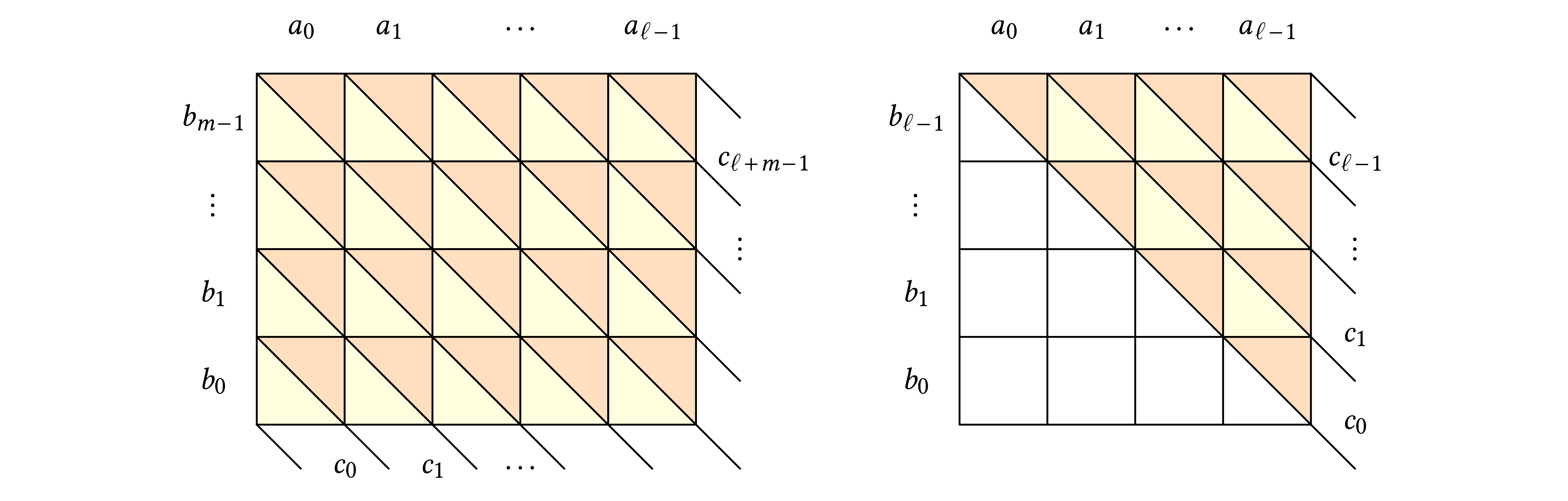
 and
and  ,
,


 as a function of
  for various multiplication schemes, as well as the
corresponding losses in bit precision. For CRTs, the bit
loss is
for various multiplication schemes, as well as the
corresponding losses in bit precision. For CRTs, the bit
loss is  for
for  or
or  and
and  ,
, for
for  .
.

 for the data fields of the SLP. Inside JIL, the data fields
are rather referred to through indices
for the data fields of the SLP. Inside JIL, the data fields
are rather referred to through indices  .
. limb
limb  limb
limb  bit
positive integer coefficients. The columns Np corresponds to
a
bit
positive integer coefficients. The columns Np corresponds to
a  bit low product, whereas the
columns Lp corresponds to a
bit low product, whereas the
columns Lp corresponds to a  bit long
product. The column AMX corresponds to the raw
bit long
product. The column AMX corresponds to the raw  bit product from the Section


 -bit
-bit moduli, using the reduction to an
  matrix product.
 using
the
using
the  using
the
using
the  )
)