Contact arithmetic  |
|
| Preliminary version of July 7, 2025 |
|
 . Grégoire
Lecerf has been supported by the French ANR-22-CE48-0016
NODE project. Joris van der Hoeven has been supported by an
ERC-2023-ADG grant for the ODELIX project (number 101142171).
. Grégoire
Lecerf has been supported by the French ANR-22-CE48-0016
NODE project. Joris van der Hoeven has been supported by an
ERC-2023-ADG grant for the ODELIX project (number 101142171).
Funded by the European Union. Views and opinions expressed are however those of the author(s) only and do not necessarily reflect those of the European Union or the European Research Council Executive Agency. Neither the European Union nor the granting authority can be held responsible for them. |
 |
 . This article has
been written using GNU TeXmacs [6].
. This article has
been written using GNU TeXmacs [6].
The irreducible factorization of polynomials over power series is central to several problems in computer algebra: integral bases, genus of a curve, Jacobian of a curve, Riemann–Roch spaces. Well-known applications include cryptography and algebraic geometry error-correcting codes. Towards solving these problems with quasi-optimal complexity, recent algorithms make use of the so-called “contact representation”. When carrying out the Newton polygon method, this allows intermediate objects to be represented in a compact way with respect to the required relative precision. In this paper, we focus on the complexity of the corresponding “contact arithmetic” and present quasi-optimal algorithms for multiplication and division in the contact representation.
|
Consider the valued field  of Laurent series over
an effective field
of Laurent series over
an effective field  . Here
“effective” means that algorithms are at our disposal for
the arithmetic operations and the zero test in . We will write
. Here
“effective” means that algorithms are at our disposal for
the arithmetic operations and the zero test in . We will write  for the
valuation on
for the
valuation on  , with value
group
, with value
group  .
.
Computing the irreducible factorization of polynomials over is central for several problems in computer algebra:
integral bases, genus of a curve, Jacobian of a curve,
Riemann–Roch spaces. Well-known applications include cryptography
and algebraic geometry error-correcting codes.
The standard way to factor polynomials over is
to use the Newton–Puiseux method. The mathematical description of
this algorithm goes back to Newton and Puiseux [16, 21]. Analyzing its computational complexity turns out to be
subtle, due to the infinite nature of Laurent series. In particular, we
must first decide how to represent and truncate elements in algebraic
extensions of .
If  is an irreducible polynomial, then
  is again a valued field and
  extends uniquely to
  . The
main goal of this paper is to device efficient algorithms for
computations with suitably truncated elements in .
. The
main goal of this paper is to device efficient algorithms for
computations with suitably truncated elements in .
If has characteristic zero, then the roots of
 are conjugate Puiseux series whose coefficients
lie in an algebraic extension of .
Taking
are conjugate Puiseux series whose coefficients
lie in an algebraic extension of .
Taking  to be one of these roots, one obvious
plan for computations in is to simply extend
by and do all our
computations with Puiseux series. However, this is non-trivial to
implement with good complexity and the restriction to characteristic
zero is an important drawback.
to be one of these roots, one obvious
plan for computations in is to simply extend
by and do all our
computations with Puiseux series. However, this is non-trivial to
implement with good complexity and the restriction to characteristic
zero is an important drawback.
In order to factor polynomials over with good
complexity, modern algorithms [12, 18–20] are based on an alternate representation for elements in
. This representation was
used by Abhyankar and Moh in [1, 2] and is
called the contact representation in [12]. The
precise definition is somewhat technical and recalled in section 1.1 below. It has the advantage of providing a compact
representation for truncations of elements of , in particular when the relative precision of such
truncations is low.
Given an ordinary non-zero Laurent series  with
with
 , its truncation with
relative precision
, its truncation with
relative precision  is simply
  . Truncating elements of
depends on the basis we choose for as a vector
space over . Consider for
instance the case when
. Truncating elements of
depends on the basis we choose for as a vector
space over . Consider for
instance the case when  and the element
  with
with  . It is
more accurate and compact to represent approximations of
. It is
more accurate and compact to represent approximations of  with respect to the basis
  than
with respect to the canonical basis
than
with respect to the canonical basis  .
Although conversions between both bases are possible, such conversions
involve a constant loss of precision, which is a problem when working
with low relative precision.
.
Although conversions between both bases are possible, such conversions
involve a constant loss of precision, which is a problem when working
with low relative precision.
In a nutshell, the contact representation is both compact and accurate
for low relative precisions, whereas the usual representation with
respect to the basis  is more straightforward and
efficient from a computational point for high precisions. In the recent
works [3, 12, 18–20],
the subtleties of the contact representation were circumvented by
keeping the precision sufficiently high; in this way, it remained
acceptable to do all actual computations using the classical
representation. However, in the case of [12], this could
only be achieved at the price of several convolutions, making part of
the algorithms less natural.
is more straightforward and
efficient from a computational point for high precisions. In the recent
works [3, 12, 18–20],
the subtleties of the contact representation were circumvented by
keeping the precision sufficiently high; in this way, it remained
acceptable to do all actual computations using the classical
representation. However, in the case of [12], this could
only be achieved at the price of several convolutions, making part of
the algorithms less natural.
The present work is inspired by the idea that, in order to design
efficient and elegant algorithms for high-level mathematical problems
(e.g. factorization over ),
it is worthwhile to find the intrinsically best adapted representation
for the underlying objects (the contact representation) and then to
first develop efficient algorithms in order to work with this
representation (contact arithmetic); see also [7].
In this paper, we present quasi-optimal algorithms for basic arithmetic
operations when using the contact representation. The contact
representation can be regarded as a hybrid one that mixes recursive
 -adic expansions (at high
relative precision) and towers of algebraic extensions (at low relative
precision). Our complexity bounds are quasi-optimal, uniformly in the
required precision. In order to achieve them, we will borrow techniques
from [9] to accelerate computations in towers of algebraic
extensions.
-adic expansions (at high
relative precision) and towers of algebraic extensions (at low relative
precision). Our complexity bounds are quasi-optimal, uniformly in the
required precision. In order to achieve them, we will borrow techniques
from [9] to accelerate computations in towers of algebraic
extensions.
The contact representation is fairly subtle, which explains the length of this paper. But we believe that this makes it even more worthwhile to separate the “low-level” contact arithmetic that we develop here from high-level applications to factorization and other problems (which we intend to work out in upcoming work).
In order to present our main result we need several definitions for the
contact representation of elements of .
 consists of:
Variables  , called
contact coordinates;
, called
contact coordinates;
Defining polynomials  for
for  ;
;
Rational numbers  ,
called contact slopes.
,
called contact slopes.
These data are required to satisfy the following properties:
Regarded in  , the
polynomial
, the
polynomial  is monic in
  of degree
  ;
;
 , for
, for  and
and  ;
;
 and
and  for ;
for ;
We endow  with the weighted valuation
defined by
with the weighted valuation
defined by  and
and  for
. We demand that:
for
. We demand that:
 , for ;
 , for .
The tower is said to be almost reduced
when  for
for  .
We write
.
We write  for
for  .
.
The above contact tower defines the following sequence of isomorphic
 -algebras:

see [12, Lemma 3.15]. Note that [12] defines
 over
over  ,
but the results from there can naturally be restated over instead. An element
,
but the results from there can naturally be restated over instead. An element  in admits a unique representative, called
canonical, in the form of a polynomial in
in admits a unique representative, called
canonical, in the form of a polynomial in  whose partial degree in
  is
is  for
for  ; see
[12, section 3.5]. We write
; see
[12, section 3.5]. We write  for the
elements of
for the
elements of  whose canonical representative has
degree
whose canonical representative has
degree  in
in  .
We let
.
We let

Following [12, Proposition 3.22], the valuation  extends to a semi-valuation
  defined by
  for
for  ,
and such that inherits the above weighted
grading of
,
and such that inherits the above weighted
grading of  . Most of the
valuations considered in this paper will be semi-valuations, so we will
drop the prefix “semi” for convenience.
. Most of the
valuations considered in this paper will be semi-valuations, so we will
drop the prefix “semi” for convenience.
The initial inverse of  is a
homogeneous element
is a
homogeneous element  such that:
 ,
,
the homogeneous component of valuation  of
of
 , written
  , equals
  .
.
Note that in [12, Definition 4.2 and Lemma 4.3] we forced a
normalized form to represent initial inverses. This normalization is not
needed in this paper because we perform computations in contact towers
directly over instead of .
 as in
Definition 1.1 is said to be
separable when
as in
Definition 1.1 is said to be
separable when  is
initially invertible in ,
for
is
initially invertible in ,
for  . It is said to be
effectively separable if the initial inverse
of the is known for algorithmic purposes, for
.
. It is said to be
effectively separable if the initial inverse
of the is known for algorithmic purposes, for
.
is said to be
regular when  has
valuation
has
valuation  and is initially invertible, for
. It is said to be
effectively regular if the initial inverse
of is known for algorithmic purposes, for
.
and is initially invertible, for
. It is said to be
effectively regular if the initial inverse
of is known for algorithmic purposes, for
.
We denote by  the -vector
space of the elements of having valuation
the -vector
space of the elements of having valuation  and (weighted) degree
  .
For
.
For  , we also write
  for the sum of the terms of that
belong to . For complexity
estimates we often use the soft-Oh notation:
for the sum of the terms of that
belong to . For complexity
estimates we often use the soft-Oh notation:  means that
  ; see [4,
chapter 25, section 7] for technical details. An algebraic complexity
model (e.g. straight-line programs) will be used for counting
operations in .
; see [4,
chapter 25, section 7] for technical details. An algebraic complexity
model (e.g. straight-line programs) will be used for counting
operations in .
For  , there exists a unique
integer
, there exists a unique
integer  such that
  equals
 ; see [12,
section 3.1]. The (logarithmic) height of a rational number
; see [12,
section 3.1]. The (logarithmic) height of a rational number  is defined by

where  represents the natural logarithm. The
number of bits for storing in a dense fashion is
asymptotically proportional to
represents the natural logarithm. The
number of bits for storing in a dense fashion is
asymptotically proportional to  .
Elements in a contact tower will be represented by the mixed
dense-sparse representation described in section 2.3. A
contact polynomial
.
Elements in a contact tower will be represented by the mixed
dense-sparse representation described in section 2.3. A
contact polynomial  is said to be
clustered if its canonical representative is monic in
of degree
is said to be
clustered if its canonical representative is monic in
of degree  (that is
  ) and
) and  .
The definitions of the quotient and remainder of contact polynomials,
written
.
The definitions of the quotient and remainder of contact polynomials,
written  and
and  ,
are recalled in section 3.1. With these conventions, we are
now able to state our main result.
,
are recalled in section 3.1. With these conventions, we are
now able to state our main result.
 (thought to be arbitrarily small).
Given an almost reduced effectively separable and regular contact
tower and
(thought to be arbitrarily small).
Given an almost reduced effectively separable and regular contact
tower and  ,
we can compute auxiliary data (that only depend on the tower and
,
we can compute auxiliary data (that only depend on the tower and  ) using

operations in  , such
that, for any
, such
that, for any  , the
following tasks can be performed using
, the
following tasks can be performed using

operations in :
given  and
and  ,
compute
,
compute  ,
,
given  and
clustered of degree
and
clustered of degree  ,
compute
,
compute  and
and  .
.
Theorem 1.4 contains the first nearly linear complexity
bound for computing in contact towers. This result relies on our
previous fast algorithms for algebraic towers [9, 10].
We are not aware of any other method with subquadratic complexity. Of
course, when the relative precision is sufficiently large, a known fast
strategy is to always work with respect to the plain coordinates  , modulo appropriate conversions;
see [12, section 3.6].
, modulo appropriate conversions;
see [12, section 3.6].
Let be irreducible in  . In characteristic zero or
  , rational Puiseux expansions can be computed
efficiently [18], hence
, rational Puiseux expansions can be computed
efficiently [18], hence  becomes
explicitly isomorphic to
becomes
explicitly isomorphic to  ,
where
,
where  is algebraic over
of degree
is algebraic over
of degree  . In this way,
arithmetic operations in
. In this way,
arithmetic operations in  can be achieved in
softly linear time. The extension of this approach is tedious for small
characteristic: Puiseux expansions do not exist any longer and
uniformizing parameters are not known to be computable in quasi-linear
time so far.
can be achieved in
softly linear time. The extension of this approach is tedious for small
characteristic: Puiseux expansions do not exist any longer and
uniformizing parameters are not known to be computable in quasi-linear
time so far.
Contact towers (a term coined in [12]) constitute an
alternate approach, that goes back to Mac Lane [15] and
that has been independently popularized by Abhyankar and Moh [1,
2] in the seventies. In fact, the latter authors designed
specific contact towers from so-called approximate roots of
, that can be computed
easily. Poteaux and Weimann achieved a quasi-linear complexity bound for
irreducibility testing [19]. Compared to Puiseux
expansions, contact towers yield more convenient algorithmic and
geometric views for germs of plane curves (the geometric counterpart of
polynomials over power series).
Puiseux expansions and contact towers are central tools for computing local irreducible factorizations. Unless the characteristic is too small, fast algorithms have been recently presented in [3, 12, 19, 20], to which we also refer for further bibliographical references.
The paper divides into two parts: up to section 5 we gather definitions and design rather elementary (but new) algorithms for contact towers and sparse arithmetic, and from section 6 we focus on fast operations.
More precisely, the next section gathers notations and prerequisites
about algorithms for multivariate polynomials and power series that are
truncated with respect to a weighted valuation. In section 3
we design elementary algorithms for contact towers. We assume that
algorithms are known for some  with
with  and we reduce computations in to
operations in . Overall we
achieve a product in whose cost grows with
and we reduce computations in to
operations in . Overall we
achieve a product in whose cost grows with  times the square of the input of the multiplicands.
The goal of the next sections is the construction of another tower that
is isomorphic to but with a sufficiently small
height with respect to its degree
times the square of the input of the multiplicands.
The goal of the next sections is the construction of another tower that
is isomorphic to but with a sufficiently small
height with respect to its degree  .
.
Let  represent the initial form of , that is its homogenous component of lowest
valuation. In section 4 we show how to compute a univariate
representation of
represent the initial form of , that is its homogenous component of lowest
valuation. In section 4 we show how to compute a univariate
representation of

over

in terms of an invertible primitive element of valuation
 .
We will call this a
univariate-valued
representation in terms of a
primitive-valued
element
.
We will call this a
univariate-valued
representation in terms of a
primitive-valued
element
1.1. Such an element is sometimes called a uniformizing parameter or a local parameter. Our terminology tries to convey the idea that this is a primitive element both for the algebraic and valuative structures.
whenever

in order to obtain a univariate-valued representation of over at precision .
We introduce flattenings in section 6: they consists in replacing consecutive levels of small degrees in a contact tower by a single level in a flattening. The problem is much more intricate than for algebraic towers [9]: a first type of flattening computes a univariate-valued representation, a second type is more straightforward to build but conversions to this representation induce a loss of precision. In addition we will design a specific fast flattened multiplication algorithm based on sparse arithmetic.
The different types of flattenings used in this article are presented in
section 7. The first type will handle the case where  and
and  so
so  and
and  hold at relative precision
in . We will show that
computing in at relative precision is equivalent to computing in
hold at relative precision
in . We will show that
computing in at relative precision is equivalent to computing in  . By means of the univariate-valued representation
introduced in section 5, we will then construct an
isomorphism between and
. By means of the univariate-valued representation
introduced in section 5, we will then construct an
isomorphism between and

where  is primitive-valued for
over
is primitive-valued for
over  and
and  is its minimal
polynomial. It will be sufficient to perform these computations using a
number of operations in that remains polynomial
in
is its minimal
polynomial. It will be sufficient to perform these computations using a
number of operations in that remains polynomial
in  . In fact
represents the degree of the underlying flattening and it will be chosen
of magnitude
. In fact
represents the degree of the underlying flattening and it will be chosen
of magnitude  , where
  can be fixed arbitrarily small. Conversions between
and
can be fixed arbitrarily small. Conversions between
and  will be performed
without increasing the current precision .
will be performed
without increasing the current precision .
For the second type of flattening, we will replace
by  , where
  is constructed as follows:
  and
and

for  . The conversions between
and will be done fast,
but with a loss of precision of order
. The conversions between
and will be done fast,
but with a loss of precision of order  .
So, once again, this flattening will be used only when
.
So, once again, this flattening will be used only when  . The special case where
  was treated before in [12, section 3.5] and corresponds to
conversions between contact and plain coordinates.
was treated before in [12, section 3.5] and corresponds to
conversions between contact and plain coordinates.
Finally, the top level algorithms are presented in section 8, where we describe a strategy to build efficient flattenings.
In this section we first gather notations and known facts about weighted multivariate polynomials and series. Then we design fast algorithms for multiplying truncated weighted polynomials.
Let be a commutative ring endowed with a
(semi-)valuation , whose
valuation group is  for some
  . Let
. Let  be
indeterminates. For any positive integers
be
indeterminates. For any positive integers  ,
we define
,
we define

For  , we assign the weight
 to and write
  for the corresponding weighted valuation of
  , that is

for all  . As in the above
context of contact towers (where and
. As in the above
context of contact towers (where and  ) we define
 |
(2.1) |
with . Since  divides
  we can set
  for
. Given
for
. Given  and
and  we write

for the -module of
polynomials of valuation that are defined up to
valuation  , which means that
two polynomials coincide in
, which means that
two polynomials coincide in  whenever their
difference has valuation
whenever their
difference has valuation  .
.
Since  for ,
we have
for ,
we have  and since the denominator of
  is we have
 |
(2.2) |
A sparse representation of a polynomial in  is a data structure that only
stores the non-zero terms of .
The support of is the set of
its monomials having a non-zero coefficient. Each such term is a pair
made of a coefficient and a degree vector. In an algebraic complexity
model the bit size of the exponents counts for free, and the relevant
size of such a polynomial is the cardinality of its support.
is a data structure that only
stores the non-zero terms of .
The support of is the set of
its monomials having a non-zero coefficient. Each such term is a pair
made of a coefficient and a degree vector. In an algebraic complexity
model the bit size of the exponents counts for free, and the relevant
size of such a polynomial is the cardinality of its support.
Consider two polynomials and  of in sparse representation. An extensive
literature exists about the general problem of multiplying and ; see [17] for a recent survey. In this paper, a superset
of in sparse representation. An extensive
literature exists about the general problem of multiplying and ; see [17] for a recent survey. In this paper, a superset  of the support of
  will always be
known and we will rely on the following classical result.
will always be
known and we will rely on the following classical result.
be positive integers
and let  be of multiplicative order
  . Let
. Let  be
a subset of
be
a subset of  , and let

The value of  and the set
  of all products
  for
for  can be computed using
  operations in .
Assume that has been precomputed. Let
be in  ,
in sparse representation, and with a support included in . All the values of
,
in sparse representation, and with a support included in . All the values of  at
at  can be computed
using
can be computed
using  operations in .
Assume that has been precomputed. Given
 in ,
there exists a unique polynomial with
support in such that
in ,
there exists a unique polynomial with
support in such that  , for
, for  .
This polynomial can be computed using
operations in .
.
This polynomial can be computed using
operations in .
Proof. The first statement is straightforward by
means of binary powering. The second and third ones are adapted from [8, section 5.2].
As said, handling supports of sparse polynomials does not matter from
the algebraic complexity point of view. Nevertheless in the rest of this
subsection we provide the reader with a few bit complexity bounds for
building prescribed sparse supports but also for computing with sparse
polynomials. The bit complexity is estimated for a RAM model over a
fixed  , as in [4].
These analyses aim at showing that the algebraic complexity bounds of
this paper might be turned into bit complexity bounds. Yet a complete
proof is out of the scope of this paper. We begin with the support of
truncated polynomials in one variable.
, as in [4].
These analyses aim at showing that the algebraic complexity bounds of
this paper might be turned into bit complexity bounds. Yet a complete
proof is out of the scope of this paper. We begin with the support of
truncated polynomials in one variable.
 ,
,  and
and  . Then
there exists a subset
. Then
there exists a subset

of cardinality  such that for all
polynomials
such that for all
polynomials

we have  whenever
  . The set
  can be computed
using
can be computed
using

bit operations.
Proof. If  then we take
 . Otherwise there exists an
integer
. Otherwise there exists an
integer  such that
  .
If
.
If  , that is
  , then
  is zero whenever
 , or equivalently whenever
 |
(2.3) |
By  is coprime with
  ,
so the condition
,
so the condition  , where

so we take

Since  the cardinality of
is
the cardinality of
is  . Computing the value of
 takes
takes  bit operations.
Then the construction of takes
bit operations.
Then the construction of takes

additional bit operations. If  ,
then we take
,
then we take

whose cardinality is  . From
the value of computed for
. From
the value of computed for  , we deduce the one for
  as
as
 using
using  bit operations, so
the total time is as claimed.
bit operations, so
the total time is as claimed.
Here the support of a set of polynomials means the union of the supports
of the polynomials in this set. So, Lemma 2.2 means that
the support of  is a set of monomials in
  of cardinality .
We extend this result to several variables. Monomials in are represented by vectors in
of cardinality .
We extend this result to several variables. Monomials in are represented by vectors in  and
supports are sequences of monomials.
and
supports are sequences of monomials.
 for
for  ,
let
,
let  , and let
  . The support of
  has
cardinality
has
cardinality

and can be computed using

bit operations.
Proof. A homogeneous polynomial in  has
has  non-zero terms by Lemma 2.2. A straightforward induction on
  yields that any homogeneous polynomial
  in
in  has at most
  non-zero terms.
If the polynomial is not homogeneous and if
 , then the number of non-zero
terms is
, then the number of non-zero
terms is  . If then the bound on the number of monomials is clear.
In order to compute the support of  we begin by
computing
we begin by
computing  ,
,  , and
, and  ,
for using
,
for using

bit operations, by  is the smallest nonnegative integer such that
  or equivalently that
  .
By
.
By  is coprime with
  ,
so we obtain
,
so we obtain

in time  . Without loss of
generality we can replace by
. Without loss of
generality we can replace by  and by
  for computing
supports. Let us write
for computing
supports. Let us write

where

Recursively we compute the support of  for
for  , and deduce the support of in time

Let  denote the cost for computing the support of
a homogeneous polynomial in .
We have shown that
denote the cost for computing the support of
a homogeneous polynomial in .
We have shown that

Unrolling this recurrence yields

For the next homogeneous component, of valuation  , we replace
  by
by  and restart the computation of the support. Consequently,
for we need to compute the support of
and restart the computation of the support. Consequently,
for we need to compute the support of  homogeneous polynomials.
For a truncated polynomial in  we use a mixed dense-sparse representation. Precisely, we store
  and the sequence of homogeneous components

where each  is stored as the sparse
representation of its specialization at
is stored as the sparse
representation of its specialization at  ,
that belongs to .
,
that belongs to .
for ,
let , and let . The support with respect to  of has cardinality
  and can be computed using

bit operations.
Proof. We adapt the proof of Lemma 2.3,
with . Let  . Each homogeneous component of has
  monomials in
  . A polynomial with relative precision has
  homogeneous
components.
homogeneous
components.
Given and ,
we will use the dense-sparse representation to multiply polynomials

efficiently. Note that  .
.
for , two polynomials  and
and
 can be multiplied using

operations in  and
and  bit operations.
Proof. Let  ,
,
 , and
, and

For  , we write
  for the support of
  where
where  is specialized at
  .
Since
.
Since  , it suffices to
compute the for
, it suffices to
compute the for  .
By Lemma 2.4, this takes
.
By Lemma 2.4, this takes
 |
|||
 |
 |
(using |
bit operations, and we have  .
.
Assume that we are given an element of
multiplicative order  , so we
apply Proposition 2.1 with
, so we
apply Proposition 2.1 with  instead
of
instead
of  . For each , we compute
  and the
set
and the
set  corresponding to
using
corresponding to
using

operations in . Then we
define

that belongs to  . We define
 similarly. By Proposition 2.1 we
compute
similarly. By Proposition 2.1 we
compute  and
and  for
for  using
using

We compute  for at
relative precision using
for at
relative precision using

operations in . Then we
interpolate  from
from  using
Proposition 2.1 again.
using
Proposition 2.1 again.
Finally, if we are not given an element of
multiplicative order , then
we appeal to [11, Proposition A.2]: the overhead only
induces logarithmic factors in the complexity bound.
Given a contact tower as in Definition 1.1, we are
interested in computing the product of two elements  and
and  in with relative
precision
in with relative
precision  . This section is
devoted to relatively simple algorithms, on which the faster ones of
section 7 will rely.
. This section is
devoted to relatively simple algorithms, on which the faster ones of
section 7 will rely.
As a first observation, since we are interested in computing with
relative precision in , we show that the defining polynomial  can be replaced by in the
definition of whenever
can be replaced by in the
definition of whenever  holds. For this purpose we introduce integers
  in
in
 and the generalized contact
tower
and the generalized contact
tower

Generalized contact towers share many of the properties of contact towers. We gather the results needed in the sequel, along with brief proofs adapted from [12].
,
any  admits a unique representative of the
form
admits a unique representative of the
form

which we call the canonical
representative of .
Proof. Assume that the polynomial , written as above, belongs to the ideal

If is not identically zero, then its initial
form  is non-zero. The proof of [12,
Lemma 3.7] extends to
is non-zero. The proof of [12,
Lemma 3.7] extends to  mutatis mutandis
and gives us that
mutatis mutandis
and gives us that

Finally [12, Lemma 3.4] implies that
must be zero, that is a contradiction.
Proof. By routine adaptation of the proof of [12, Proposition 3.22].
The integer defined by

is called the ramification index of  and
and  , for
, for  . From Definition 1.1 it is clear
that divides
. From Definition 1.1 it is clear
that divides  .
By construction, divides , and
.
By construction, divides , and

divides  , for .
Elements in  will be called generalized
contact polynomials. Such a polynomial
will be usually written
will be called generalized
contact polynomials. Such a polynomial
will be usually written

with  and
and  .
This is called the contact representation of . The integer
is called the degree of in and is written
.
This is called the contact representation of . The integer
is called the degree of in and is written  .
We will write
.
We will write  for the set of contact polynomials
of of degree in . A contact polynomial
for the set of contact polynomials
of of degree in . A contact polynomial  is said to be clustered if its canonical
representative is monic in of degree (that is ) and
is said to be clustered if its canonical
representative is monic in of degree (that is ) and
 . Note that
is clustered in
. Note that
is clustered in  .
.
Let and be contact
polynomials in , if is clustered of degree  ,
then there exist unique elements
,
then there exist unique elements  such that

This decomposition is adapted from [12, Lemma 3.12] and
yields a natural notion of division: there exists unique contact
polynomials  and
and  such
that
such
that

The quotient is written  and the remainder
  is written
  .
.
Now let  and
and  be contact
polynomials in and let us compute their product
be contact
polynomials in and let us compute their product
 , where

Each  writes canonically into
  with
with  and
and  in
in  . Now if
  ,
then we have
,
then we have

In other words, computing in
is the same as in when  and
and  . By decreasing induction
on
. By decreasing induction
on  , it follows that
computing in is the same
as in where we set
, it follows that
computing in is the same
as in where we set  when
, and
when
, and  otherwise for .
The rest of this section is devoted to rather elementary algorithms for
multiplying elements in a generalized contact tower at a given relative
precision . In order to keep
the notation simple, we drop the superscript for
generalized contact towers. So, unless specified, contact towers will be
of the generalized kind.
Given a clustered contact polynomial  of degree
in ,
its pre-inverse will refer to the clustered contact
polynomial
of degree
in ,
its pre-inverse will refer to the clustered contact
polynomial  of degree in
such that
of degree in
such that

Since  holds for all
  , if a pre-inverse exists, then it is necessarily
unique. The existence of pre-inverses is addressed in section 3.5.
We introduce the following cost functions:
, if a pre-inverse exists, then it is necessarily
unique. The existence of pre-inverses is addressed in section 3.5.
We introduce the following cost functions:
 is a function that bounds the cost for
adding two elements in of degree in with relative precision
is a function that bounds the cost for
adding two elements in of degree in with relative precision
 .
.
 is a function that bounds the cost for
multiplying two elements in of degree in with relative
precision .
is a function that bounds the cost for
multiplying two elements in of degree in with relative
precision .
 bounds the cost of a division in of a contact polynomial of degree
  by a clustered contact polynomial of of
degree with relative precision .
by a clustered contact polynomial of of
degree with relative precision .
 bounds the cost for computing the
pre-inverse of a clustered contact polynomial in
of degree in with
relative precision .
bounds the cost for computing the
pre-inverse of a clustered contact polynomial in
of degree in with
relative precision .
 .
.
Proof. Let  and
and  be in
be in  .
Regarded in
.
Regarded in  their product
  costs
costs  . We divide by
  in with
 operations. Let
  and
and  denote the resulting quotient
and remainder, so
denote the resulting quotient
and remainder, so  . Since
has valuation
. Since
has valuation  ,
and since
,
and since  , we have

 be a clustered polynomial in of degree
  in , together with its pre-inverse
  . For all
  at relative
precision
at relative
precision  , there exists a
unique
, there exists a
unique  such that
 |
(3.1) |
It is given by  .
.
Proof. Equation and  such that

which implies that

so is the unique solution of Equation
The following simple multiplication algorithm in
makes use of operations in ,
whose cost functions are assumed to be as in section 3.2.
Algorithm
For 
compute  .
.
Return  .
.
Proof. The correctness is straightforward from
the definitions. The number of non-zero terms in
is  by Lemma 2.2. The number of
non-zero products
by Lemma 2.2. The number of
non-zero products  performed in step 1 is
therefore
performed in step 1 is
therefore  , so this step
costs
, so this step
costs

thanks to Lemma 3.3. Step 2 takes

operations in . Since , we use  in
order to simply the final cost bound.
in
order to simply the final cost bound.
Let  be a clustered polynomial of degree in and let . We address the computation of the quotient
 and the remainder of
  at
relative precision . We
assume that the pre-inverse
at
relative precision . We
assume that the pre-inverse  of
of  is at our disposal at relative precision .
Algorithm
Set  .
.
For  from
from  down to
do:
down to
do:
Compute  , where
represents the coefficient of
, where
represents the coefficient of  in the contact representation of ;
Replace by  .
.
Return  and .
and .
Proof. For a fixed value of  in step 2, by Lemma 3.4, we have

so the algorithm finishes with the expected quotient and remainder. The
number of non-zero coefficients encountered
during step 2 is by Lemma 2.2.
According to Lemma 3.3, step 2.a costs  . Step 2.b costs

Finally we use .
Given clustered of degree
in , we wish to compute its
pre-inverse  with relative precision . We adapt the well-known method for power
series inversion. The algorithm is recursive on the height . If
with relative precision . We adapt the well-known method for power
series inversion. The algorithm is recursive on the height . If  then the
pre-inverse of
then the
pre-inverse of  is
is  because
  .
.
 is the pre-inverse of
  regarded as a clustered polynomial in
of degree
regarded as a clustered polynomial in
of degree  in
in  and at
relative precision ,
then
and at
relative precision ,
then

is the pre-inverse of at relative precision
.
Proof. Since  ,
is clustered in ,
so is well defined. Computing the pre-inverse of
means finding
,
is clustered in ,
so is well defined. Computing the pre-inverse of
means finding  such that

This condition is equivalent to

that is further equivalent to

in , then to

and finally to

From Lemma 3.4 we deduce that  .
.
 and let
  be
clustered of degree in
such that
be
clustered of degree in
such that

There exists a unique  such that

It is given by

where  is the coefficient of
  in and
  is defined by

Proof. From

the condition for  is equivalent to

Since  is the pre-inverse of
at relative precision , there
exists a unique solution for given by Lemma 3.4.
is the pre-inverse of
at relative precision , there
exists a unique solution for given by Lemma 3.4.
A straightforward induction based on the two latter lemmas shows that pre-inverses do exist.
of degree
in can be computed at relative precision using

operations in .
Proof. From Lemmas 3.7 and 3.3 we can compute the pre-inverse of

at relative precision using

operations in . By induction
on , suppose that the
pre-inverse of  is known
along with the product
is known
along with the product  , for
some
, for
some  and still at relative precision . Thanks to Lemma 3.8
we deduce the pre-inverse
and still at relative precision . Thanks to Lemma 3.8
we deduce the pre-inverse  of
of  in the form

with a cost . The product

at relative precision costs

By taking the sum of these costs for  and for
when is known to be non-zero at relative
precision , we achieve the
total bound
and for
when is known to be non-zero at relative
precision , we achieve the
total bound

for the pre-inverse of .
Finally we use in order to simplify this
bound.
 to
to
So far we have reduced operations in to
operations in . Now we
proceed by induction in order to reduce operations in
to operations in for any fixed .
Proof. If  then
then

Otherwise we have  , hence

 ,
, , and let be a clustered
polynomial of degree in . Let
,
, , and let be a clustered
polynomial of degree in . Let  denote the
coefficient of
denote the
coefficient of  in . Then the pre-inverses of
  ,...,
,..., ,
can be obtained with a cost
,
can be obtained with a cost

Once these pre-inverses are known, we may compute in with the cost bound

where underlying divisions in are only
allowed by .
In addition, given the pre-inverses of ,..., we
have

Proof. From Proposition 3.5 we may take

Assuming that the pre-inverse of is known,
thanks to Proposition 3.6, for divisions by , we may take

From Lemma 2.2 we straightforwardly obtain

By summing these three inequalities and using , we deduce

By unrolling the latter inequality and using Lemma 3.10, we obtain that
whenever the pre-inverses of ,
..., , are known.
From Proposition 3.9 we know that

By using

Iterating the latter inequality yields
From Lemmas 3.3 and 3.7 the pre-inverse of
is obtained at relative precision using

operations in . Consequently,
the cost for obtaining the pre-inverses of ,
..., , is
which concludes the proof.
So far we have designed rather elementary algorithms for contact towers, that will be useful to section 7. Computing pre-inverses faster will be useful as well. The following lemma is adapted from the usual fast power series inversion method.
and be
clustered monic contact polynomials of of
degree in and let  be such that
Then for any  ,
,  is the pre-inverse of
  at
precision .
at
precision .
Proof. Let  ,
,
 ,
,  ,
,  . From

we obtain

Since  and
and  ,
we deduce that
,
we deduce that

The conclusion follows from  .
.
, let  , and let
be clustered of degree in
such that
, and let
be clustered of degree in
such that

There exists a unique  such that

It is given by

where  is defined by

Proof. From

the condition for becomes

and then

By Lemma 3.12,  is the pre-inverse
of
is the pre-inverse
of  at relative precision . There exists a unique solution for given by Lemma 3.4.
of degree
in can be computed at relative precision using

operations in whenever .
Proof. From Lemma 3.7 we can compute the pre-inverse of
at relative precision using

operations in . This makes it
possible to apply Lemma 3.13  times,
with
times,
with  , in order to obtain the
pre-inverse of using
, in order to obtain the
pre-inverse of using

operations in .
As for usual polynomials, pre-inverses are used to reduce divisions to multiplications.
be a clustered monic contact
polynomials of of degree
in , let
be its pre-inverse, and let  .
The quotient
.
The quotient  can be computed as

Proof. Let  ,
and let
,
and let  , so we have

By multiplying both sides of this equality by we
obtain

whence  .
.
be a clustered monic
contact polynomial of of degree in and given at precision . Given the pre-inverse of at precision , the division of a contact polynomial of
 at precision costs

Proof. This follows from Lemma 3.15.
Throughout this section, represents a
generalized contact tower as in Definition 1.1 and is a fixed integer. We will assume that  so that
  is a tower of algebraic
extensions. One important question is how to compute efficiently in
, provided that we know how
to compute efficiently in
is a tower of algebraic
extensions. One important question is how to compute efficiently in
, provided that we know how
to compute efficiently in  .
We will achieve this by representing elements in
as follows.
.
We will achieve this by representing elements in
as follows.
over at precision  is made of the
following data:
is made of the
following data:
a homogeneous primitive element  of over of valuation ,
an initially separable monic polynomial  of
degree , of valuation
of
degree , of valuation
 at relative precision , where
  has
valuation ,
has
valuation ,
polynomials  in
in  of
valuations
of
valuations  and at relative precision .
These data satisfy the following properties:
 ,
,
 ,
,
 , for
, for  .
.
Any element of can uniquely be represented
as an element of  via the following
isomorphism:
via the following
isomorphism:

In this section, we focus on the computation of an initial
primitive-valued representation, which is simply a
univariate-valued representation of minimal precision  . For this purpose, we define

for . Computing an initial
univariate-valued representation of over essentially amounts to computing a homogeneous
element in  of valuation
such that the map
of valuation
such that the map

is surjective. We call such a a
primitive-valued element of over  . Its minimal polynomial
  over is the monic generator of the
kernel of this map. It is homogeneous of degree . The surjectivity further implies the existence of
homogeneous polynomials
over is the monic generator of the
kernel of this map. It is homogeneous of degree . The surjectivity further implies the existence of
homogeneous polynomials  in
in  such that
  holds for . These polynomials are obtained as a byproduct of
the computation of and, together with , give rise to the desired initial
univariate-valued representation.
holds for . These polynomials are obtained as a byproduct of
the computation of and, together with , give rise to the desired initial
univariate-valued representation.
It is classical that is isomorphic to an algebra
of the form  , where
  is an algebraic extension of and
 ; see [12,
section 6]. On the level of coefficients, we are therefore led to
compute in so-called algebraic towers
; see [12,
section 6]. On the level of coefficients, we are therefore led to
compute in so-called algebraic towers  over . Some relevant complexity results
for such computations are recalled in section 4.1.
over . Some relevant complexity results
for such computations are recalled in section 4.1.
Now direct computations in can become expensive
for towers of large heights, since every next floor gives rise to a
constant overhead. This explains the interest of doing relative
computations of over : using the univariate-valued representation, this
will allow us to bundle all floors between level
and into a single univariate extension, for
which we can use fast univariate arithmetic, in the same spirit as the
accelerated tower arithmetic from [9]. In section 4.2,
we first construct an isomorphism  of the form
 where
where  and
and  . Here
  is a primitive
algebraic extension of
is a primitive
algebraic extension of  that is isomorphic to
(in particular, computations in
will be more efficient than computations in ).
that is isomorphic to
(in particular, computations in
will be more efficient than computations in ).
A natural candidate for a primitive-valued for
over is  . Although this element is not always
primitive, as we shall show in section 4.3, it turns out
that we may always take
. Although this element is not always
primitive, as we shall show in section 4.3, it turns out
that we may always take  for some suitable value
of
for some suitable value
of  in .
In section 4.4 we show how to compute , ,
and derive the desired initial primitive-valued representation of over .
in .
In section 4.4 we show how to compute , ,
and derive the desired initial primitive-valued representation of over .
Remark  be homogeneous in Definition 4.1. Nonetheless, this is
naturally the case for initial primitive-valued representations, and
this property also simplifies computations. Furthermore, it turns out
that we can keep the same primitive-valued element
when lifting our representation to higher precisions, as we will show in
section 5 below.
be homogeneous in Definition 4.1. Nonetheless, this is
naturally the case for initial primitive-valued representations, and
this property also simplifies computations. Furthermore, it turns out
that we can keep the same primitive-valued element
when lifting our representation to higher precisions, as we will show in
section 5 below.
A separable (algebraic) tower over
is a sequence with  and
and

where the  are monic separable polynomials. We
write
are monic separable polynomials. We
write  for the image of
  in
in  and set
  for . We will write

for the degree of over . The tower is said to be effectively
separable when we are further given  and
and
 in
in  of respective degree
 and
and  such that the
Bézout relation
such that the
Bézout relation

holds, for . Throughout the
rest of this paper, without loss of generality, we will freely assume
that such towers are simplified so that  holds
for . The cardinality of will be written
holds
for . The cardinality of will be written  .
We will rely on the following complexity bound.
.
We will rely on the following complexity bound.
 be a fixed positive
constant, that can be taken arbitrarily close to
be a fixed positive
constant, that can be taken arbitrarily close to  . Given an explicitly separable tower , one multiplication and one
inversion (when the inverse exists) in
costs
. Given an explicitly separable tower , one multiplication and one
inversion (when the inverse exists) in
costs

operations in .
Proof. If  ,
then the result directly follows from [10, Theorem 4].
Otherwise, with the notation of [10, section 7], we observe
that the assumption on
,
then the result directly follows from [10, Theorem 4].
Otherwise, with the notation of [10, section 7], we observe
that the assumption on  is only needed to build
primitive tower representations of degree
is only needed to build
primitive tower representations of degree  ,
so it is sufficient to assume
,
so it is sufficient to assume  instead. After
that, if
instead. After
that, if  , then we appeal to
[11, Proposition A.2]: the overhead only induces
logarithmic factors in the complexity bound.
, then we appeal to
[11, Proposition A.2]: the overhead only induces
logarithmic factors in the complexity bound.
The next lemma addresses the complexity for obtaining a univariate
representation of over
for a given . For the purpose
of this paper, this complexity bound does not need to be sharp because
 will be taken relatively small.
 and assume
  . There exist
  in ,
in ,  separable and monic of degree ,
and
separable and monic of degree ,
and  such that

is an -algebra
isomorphism and that

In addition, if we are given  distinct
elements in , then such a
univariate representation ,
distinct
elements in , then such a
univariate representation ,  ,
,
 of over can be computed using

operations in . One
conversion between and
costs  operations in .
Proof. If is a field,
then [9, Corollary 1] allows us to compute the univariate
representation of over
using  operations in
. In general, is not a field, but panoramic evaluation can be used to
simulate field operations in it. Precisely we appeal to [10,
Corollary 1] in order to run the algorithm underlying [9,
Corollary 1]: using
operations in
. In general, is not a field, but panoramic evaluation can be used to
simulate field operations in it. Precisely we appeal to [10,
Corollary 1] in order to run the algorithm underlying [9,
Corollary 1]: using
operations in , we obtain a
so-called panoramic splitting

of and univariate representations  ,
,  ,
,
 for the restrictions of
over
for the restrictions of
over  for
for  .
We further know from [10, Corollary 1] that one evaluation
of
.
We further know from [10, Corollary 1] that one evaluation
of  and
and  takes
takes  operations in .
Finally, we take
operations in .
Finally, we take  for
for  . We extend to
  coefficient-wise, and set
  and
and  for .
for .
The cost of the conversions between and is addressed in [9, Proposition 5],
which simplifies to  operations in : these conversions only involve ring
operations in , so [9,
Proposition 5] can be used even if is not a
field.
operations in : these conversions only involve ring
operations in , so [9,
Proposition 5] can be used even if is not a
field.
It is known that  decomposes into a separable
extension of followed by purely ramified
extensions; see for instance [12, section 6]. Given , we use this decomposition in
order to compute a univariate-valued representation of
over . We let
decomposes into a separable
extension of followed by purely ramified
extensions; see for instance [12, section 6]. Given , we use this decomposition in
order to compute a univariate-valued representation of
over . We let

We begin with a first technical rewriting of , summarized in the following lemma.
be an almost reduced, effectively
separable and regular contact tower, let ,
and assume that we are given distinct elements
in . Using

operations in , we can
compute the following data:
An effectively separable algebraic tower
as in section 4.1;
A univariate representation ,
 ,
of over ,
as in Lemma 4.4;
,
of over ,
as in Lemma 4.4;
 in ,
in ,
 in ,
in ,
 in
in  ,
,
 in
in  and
and  in
in  such that

is a -algebra
isomorphism, that preserves the valuation, when setting  and
and  .
.
One evaluation of  and
and  at a homogeneous element costs

operations in .
Proof. By [12, Proposition 13] we
can compute a so-called initial expansion [12, Definition
10] of , using
 |
(4.1) |
operations in . In
particular, combined with [12, Proposition 12], we obtain:
An effectively separable tower

where  is monic of degree
  in . For , the class of in is invertible and its
inverse is known.
in . For , the class of in is invertible and its
inverse is known.
For , an invertible  and its inverse, along with a -algebra isomorphism

that preserves the valuation for the weight  of
of  and such that one evaluation of
  and
and  in valuation
  with
with  costs
costs
by and
by a suitable power of  .
.
Then, we compute  invertible such that
  holds, and define the
  -algebra
isomorphism
-algebra
isomorphism

Thanks to Lemma 4.4, we may compute a univariate
representation of over
using
 |
(4.3) |
operations in . Lemma 4.4 also ensures that one conversion between
and costs
 |
(4.4) |
In particular we compute  with this cost, and
extend
with this cost, and
extend  coefficient-wise into
  :
:

Finally, we set

For  , we take
  ,
,  ,
and
,
and  such that

For , we compute  invertible in such that

where  and
and  .
Writing
.
Writing  and
and  ,
we obtain that
,
we obtain that

so we take

In this way,  products in
suffice to obtain
products in
suffice to obtain  from , that is
  products thanks to
The total cost of this construction of is the
sum of  evaluations of
  ,
,
 ,
,  of
cost
conversions from to of
cost
further products in .
of
cost
conversions from to of
cost
further products in .
When evaluating (resp. ) at a homogeneous element, the contribution of (resp. of  )
costs
)
costs  is represented uniquely in the form
 , where
  ,
,  ,
,
 ,
,  . For such an element we
have
. For such an element we
have

Therefore, one evaluation of  or
or  costs
costs
 |
(4.5) |
Finally, the cost of one evaluation of or at a homogeneous element is bounded by the sum of
Example  defined by
 ,
,  ,
,  ,
,  , and
, and

At the first level of the contact tower, we have  ,
,  , and
we take
, and
we take  , whence
  ,
,  ,
and
,
and

Since the image  of
of  in
in
 is primitive-valued, we may define

At the second level,  is rewritten
  over , whence
 and
and  .
We set
.
We set  , hence
  , and obtain

where  is the image of
  in
in
 . Taking the image
  of
of  in
in  for
a primitive-valued element, we define
for
a primitive-valued element, we define

For the third level of the contact tower,  is
rewritten
is
rewritten  over ,
whence
over ,
whence  and
and  .
We set
.
We set  and obtain

Taking the image  of
of  in
in
 for a primitive-valued element, we define

Now, let us build the map of Lemma 4.5
for  . For the univariate
representation of
. For the univariate
representation of  over
over  , we use the primitive element
  , hence

and obtain

We deduce the following expression for :

A natural candidate for a primitive element of minimal valuation for
over is . Unfortunately, it is not always primitive, as
illustrated by the following example.
Example  over is
  , which is not separable. So
  is not a primitive element of over .
We will show in the proof of Proposition 4.10 that  is indeed primitive for over
for suitable values of
in . We begin with a
technical lemma, where
is indeed primitive for over
for suitable values of
in . We begin with a
technical lemma, where  stands for a new
polynomial variable: in the context of Lemma 4.4, if
stands for a new
polynomial variable: in the context of Lemma 4.4, if  is a primitive element of
over , then
is a primitive element of
over , then  is also primitive for almost all
  .
.
 elements in , and let

where  represents the pre-image of
  in
in  .
Using
.
Using

operations in , we can
compute  ,
,  , and
, and  such that:
Proof. Let us first assume that
is a field. Given , note that
 is the minimal polynomial of
  in
in  . Therefore if
  is a root of in a suitable
algebraic closure, then
is a root of in a suitable
algebraic closure, then  is invertible if and
only if
is invertible if and
only if  is non-zero. Consequently at most values of
  do not satisfy
property
do not satisfy
property

the multiplicativity of the resultant yields

where

Since is a separable extension of , the polynomial  is
separable in
is
separable in  , and therefore
 is invertible in .
Consequently, if
is invertible in .
Consequently, if  , then the
leading term of
, then the
leading term of  is
is

If  , then
clearly has degree
, then
clearly has degree  in
in  . It follows that
  is not the
zero polynomial and that at most
is not the
zero polynomial and that at most  values of do not satisfy property
Since

there exists a suitable value for in any given
set  of cardinality
  .
In order to find a suitable value, it suffices to evaluate
.
In order to find a suitable value, it suffices to evaluate  at all the points of .
The polynomial  has degree
  in
in  and degree

in . So it can be computed
using

operations in by means of the Berkowitz
algorithm [22] applied to the Sylvester matrix of  and
and  . Since
 has degree

it can be computed using

operations in by means of the Berkowitz
algorithm.
The evaluation of at all the elements of takes  operations in ; see [4, Chapter 10]
for instance. From Proposition 4.3 we know that one
operation in reduces to
operations in . Consequently
we obtain a suitable value for using a total
number of
operations in ; see [4, Chapter 10]
for instance. From Proposition 4.3 we know that one
operation in reduces to
operations in . Consequently
we obtain a suitable value for using a total
number of  operations in .
In this way is a primitive element of , of minimal polynomial  . Therefore, there exists a unique
 satisfying property is a root of ,
then and
satisfying property is a root of ,
then and  share a proper
gcd, that is
share a proper
gcd, that is  . In this case,
it is known that this gcd is proportional to the first subresultant of
and ;
see [14, Theorem 9]. Since the specialization at
. In this case,
it is known that this gcd is proportional to the first subresultant of
and ;
see [14, Theorem 9]. Since the specialization at  of the first subresultant
  of and
  coincides with the first
subresultant of and , we deduce that
coincides with the first
subresultant of and , we deduce that  is
invertible modulo .
is
invertible modulo .
The polynomials  and
and  are
minors of the Sylvester matrix of and
are
minors of the Sylvester matrix of and  ; see [14, section
2.1] for instance. They can thus be computed using
; see [14, section
2.1] for instance. They can thus be computed using  operations in , again by
means the Berkowitz algorithm. Computing
operations in , again by
means the Berkowitz algorithm. Computing  further
needs
further
needs  operations in .
It remains to handle the case where is not a
field. Panoramic evaluation can perform the above calculations [10,
Corollary 1] still using operations in : we obtain a panoramic splitting
of and suitable values  in for the restrictions of
over for
in for the restrictions of
over for  ,
along with the corresponding
,
along with the corresponding  and
and  . We further know from [10,
Corollary 1] that one evaluation of and takes operations in . Finally we take
. We further know from [10,
Corollary 1] that one evaluation of and takes operations in . Finally we take  ,
,  ,
,
 , where
is implicitly extended to
, where
is implicitly extended to  coefficient-wise.
Example  and
and

We put Lemmas 4.5 and 4.8 together in order to
construct an initial primitive-valued element of
over , written in the following proposition.
be an almost reduced
effectively separable and regular contact tower, let , and assume that we are given distinct elements in .
Using

operations in , we can
compute:
a homogeneous polynomial in of valuation  ,
,
a monic separable homogeneous polynomial  of degree , where has valuation ,
homogeneous polynomials in of respective valuations ,
such that

and

In other words, the map

is an isomorphism of -algebras.
One evaluation of  and
and  at a homogeneous element costs

operations in .
Proof. We set

which is another -algebra
representation of via the map  introduced in the proof of Lemma 4.5. A homogeneous element
of
introduced in the proof of Lemma 4.5. A homogeneous element
of  can be written
  ,
where
,
where  ,
,  , and .
Consequently, the product of two homogeneous elements of costs
, and .
Consequently, the product of two homogeneous elements of costs  operations in .
First, we build the isomorphism of Lemma 4.5 using
 |
(4.6) |
operations in . Then, we
compute ,  , and
, and  as in Lemma 4.8, using
 |
(4.7) |
operations in . This yields
the following isomorphism of -algebras:

From Lemma 4.8, we know that is
invertible. Since  is the minimal polynomial of
modulo ,
the inverse of modulo is
given by
is the minimal polynomial of
modulo ,
the inverse of modulo is
given by

which can be obtained with ring operations in
plus the inversion of . The inverse of  modulo equals
  ,
which can be computed using further operations
in . On the other hand,
computing modulo takes
,
which can be computed using further operations
in . On the other hand,
computing modulo takes
 operations in .
A homogeneous element of  can be uniquely written
 , where
  , ,
, and . Consequently, computing
, ,
, and . Consequently, computing

takes
 |
(4.8) |
operations in . The same cost
bound applies to  .
.
The characteristic polynomial of  over is

and its computation takes
 |
(4.9) |
operations in . As seen in
the proof of Lemma 4.8, the integer
is invertible in , so  is separable, and the map

is a -algebra isomorphism.
Let us consider a homogeneous element of  ,
of the form
,
of the form

where  , ,
, ,  ,
,
 , and
, and  is independent of . The
computation of
is independent of . The
computation of

takes
 |
(4.10) |
operations in . By reverting
these calculations, the same cost is achieved for one evaluation of
 . We extend the map
  to
to  coefficientwise, and compute

Composed with , we finally
obtain the desired initial univariate-valued representation of over :

The total cost of the construction of Y,  ,
,
 , and
is bounded by the sum of
, and
is bounded by the sum of
operations in . The cost of
one evaluation of  or
or  is
at most by the sum of
is
at most by the sum of  , and the costs for and given in Lemma 4.5,
that is bounded by
, and the costs for and given in Lemma 4.5,
that is bounded by
operations in . Finally we
take  and
and  ,
for .
,
for .
Example over given in Proposition 4.10. The initial primitive-valued element is

and the corresponding initial univariate-valued representation is

In this section we consider a generalized contact tower
as in section 3.1 and an index such
that

It follows that has dimension
over , and that has dimension  over . We are interested in computing a
primitive-valued element representation of over
.
over . We are interested in computing a
primitive-valued element representation of over
.
Using Proposition 4.10, we first compute an initial
univariate-valued representation of  over
over  . This yields a homogeneous
polynomial in of
valuation , a monic separable
homogeneous polynomial of degree , where has valuation
, and homogeneous polynomials
in of respective
valuation , such that
. This yields a homogeneous
polynomial in of
valuation , a monic separable
homogeneous polynomial of degree , where has valuation
, and homogeneous polynomials
in of respective
valuation , such that

and

Then, given a target precision ,
we will use a suitable Hensel lifting in order to obtain  monic of degree ,
and polynomials
monic of degree ,
and polynomials  in such
that:
in such
that:
 , and
, and  , for ,


We begin by presenting our lifting strategy, which is naturally based on
the Newton operator of the map  .
.
Let  denote a commutative ring, let
  and let
  be independent variables.
Expanding
be independent variables.
Expanding

in terms of the powers of  in
in  yields
 |
(5.1) |
where  are polynomials in
  of total degree
  . This
operator
. This
operator  is usually called the Hasse
derivative of orders
is usually called the Hasse
derivative of orders  .
Applied to a monomial
.
Applied to a monomial  , where
 , we have

Note that

For any  , the following
Taylor expansion holds after replacing
, the following
Taylor expansion holds after replacing  by
by  in
in
 |
(5.2) |
Consider the map

whose Jacobian matrix is

The corresponding Newton iterator is the map

In order to quantify the convergence of this operator, we begin by
studying the valuations of the determinant and the adjunct matrix of
 .
.
Proof. For simplicity, the proof is presented
for and  .
The general case only involves syntactic adjustments. The usual
expansion of the determinant of
.
The general case only involves syntactic adjustments. The usual
expansion of the determinant of  yields
 |
(5.3) |
where  is the permutation group of
  ,
,  represents the usual
signature function, and
represents the usual
signature function, and  stands for the entry
 in .
Note that a product
in .
Note that a product  vanishes whenever
  for some in
  , and that the identity permutation
  is the only element of that satisfies
  for all .
Now let  denote the subset of permutations that satisfy
  for all
  and such that the latter inequality is an equality
for exactly values of . The expansion
and such that the latter inequality is an equality
for exactly values of . The expansion

The valuation of the first term equals  .
For
.
For  and
and  ,
we have
,
we have

which concludes the proof.
Proof. The entry  of
of  is
is  times the
  -minor
  of . When
  ,
we have
,
we have
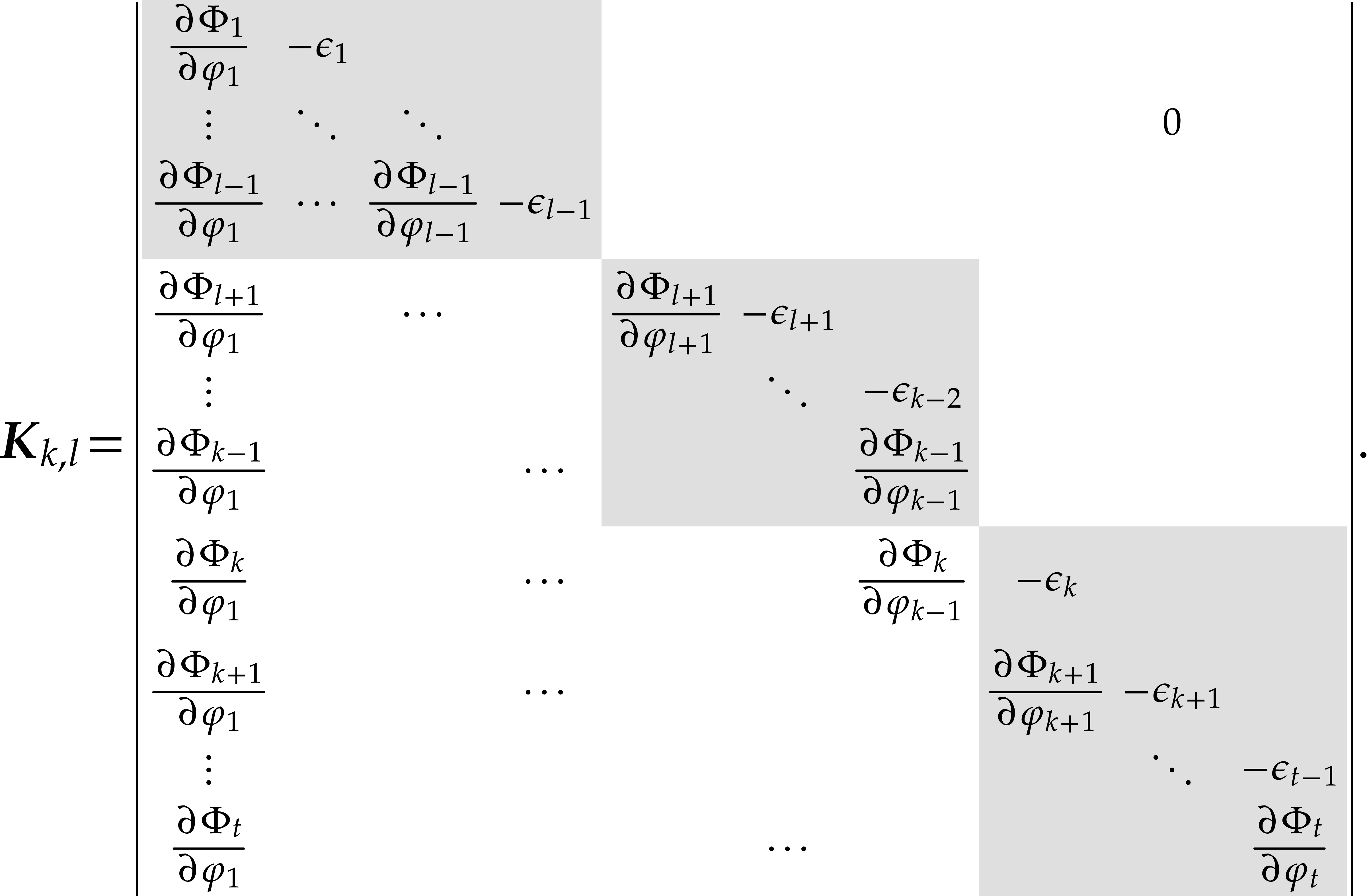 |
(5.4) |
Let  denote the set of bijections

such that ,  (resp.
  ,
,  ) is the number of indices
  (resp.
  ,
,  ) such that
  .
We expand the determinant
.
We expand the determinant

Then for all  we verify that

Thanks to Lemma 5.1, this concludes the proof of the lemma
when . If  , then the determinant
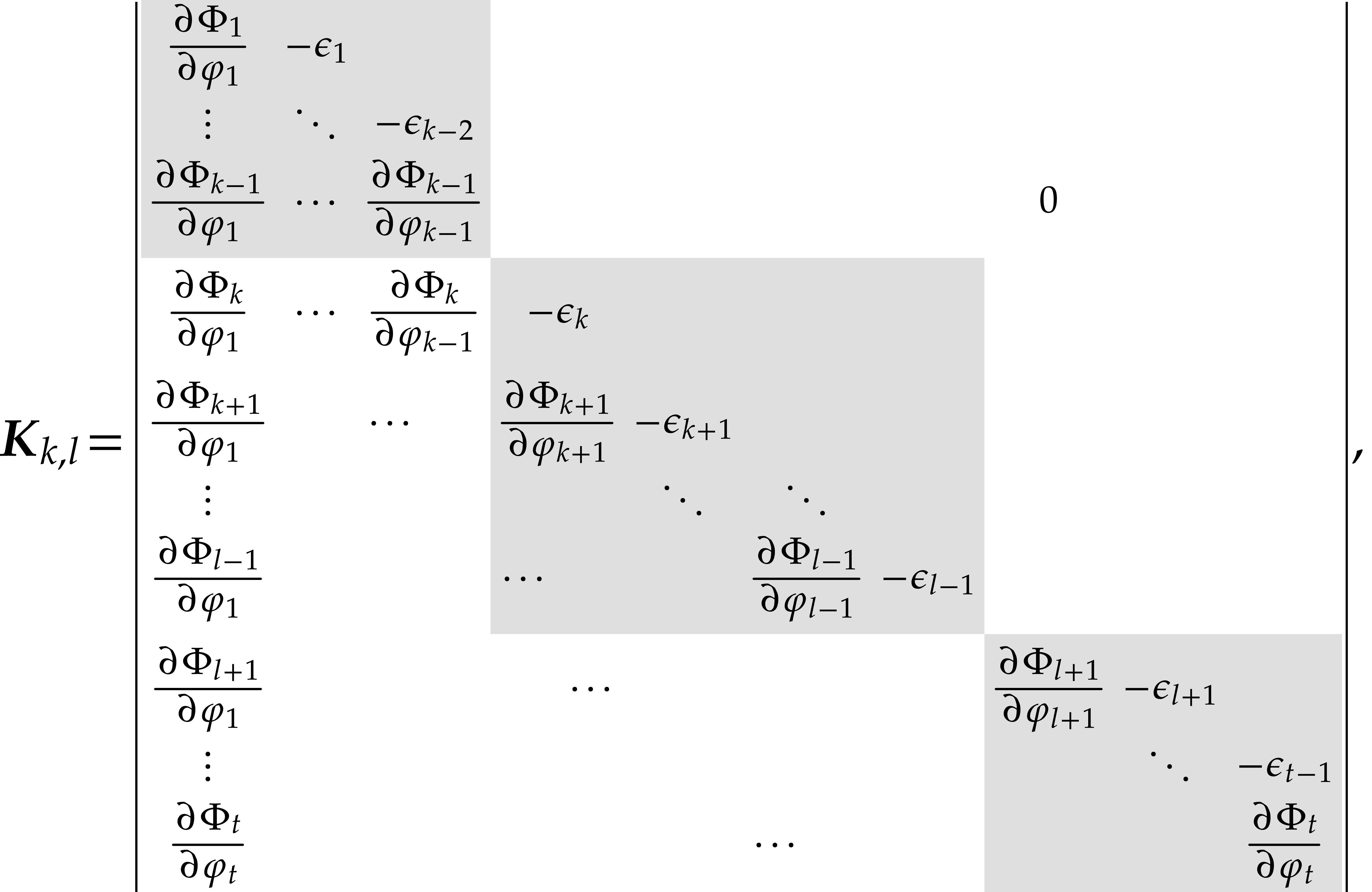
is block triangular (with three blocks). Applying Lemma 5.1 to the first and third blocks, we obtain

It follows that

since  .
.
The above valuation estimates now allow us to study of the behavior of
the Newton operator of  from precision
  to
to  . For this
purpose, let be a valued algebra over . For ,
let
. For this
purpose, let be a valued algebra over . For ,
let  be such that

and  is invertible of valuation
  . Still for ,
we are looking for
. Still for ,
we are looking for  such that
  and
and
 |
(5.5) |
Setting  , the first order
Taylor expansion of
, the first order
Taylor expansion of  yields
where  represents the sum of the terms of order
at least
represents the sum of the terms of order
at least  :
:

Since  and
and  ,
for , we have
,
for , we have

After left multiplying both sides of  , we obtain that

Regarding “” and
“ ”
component-wise, Lemma 5.2 yields
”
component-wise, Lemma 5.2 yields

and

It follows that

Consequently, under the constraints on the valuations of the  , equations
 |
(5.7) |
Finally we have shown that the  exist and are
uniquely determined by
exist and are
uniquely determined by

In other words

is the unique solution of
We are now ready to extend Proposition 4.10 for the computation of univariate-valued representations at higher precisions. The following algorithm is adapted from [5, Section 4].
Algorithm
Compute  as in Proposition 4.10
and let
as in Proposition 4.10
and let  .
.
While  do:
do:
Compute  modulo
  at relative precision as
 .
.
Compute  , for
.
, for
.
 .
.
Compute  .
.
For , compute
 .
.
Replace by  , by
, by  and
and  by
by  , for .
Return .
is almost reduced, then it performs

operations in . In
addition, the polynomials  of a
univariate-valued representation are uniquely determined at precision
by the contact tower
and the choice of . The
constant coefficient
of a
univariate-valued representation are uniquely determined at precision
by the contact tower
and the choice of . The
constant coefficient  is initially invertible
in of valuation .
is initially invertible
in of valuation .
Proof. Let

and let  be the extension of
  to
to  , so
, so  . Proposition 4.10 gives us a
univariate-valued representation at precision
. Proposition 4.10 gives us a
univariate-valued representation at precision  . Note that is homogeneous,
and that
. Note that is homogeneous,
and that  and the are
uniquely determined by the choice of at this
precision.
and the are
uniquely determined by the choice of at this
precision.
In step 2.a, the Newton iteration

Note that  , for . At the end of step 2.b, we obtain
  and
and

for . The  are uniquely determined by these properties, under the constraints on
the valuation of the
are uniquely determined by these properties, under the constraints on
the valuation of the  .
.
By construction,  has valuation
  and therefore
  coincide with
at precision
coincide with
at precision  . It follows
that
. It follows
that

and that

for . It follows that

holds for , and similarly
that

This proves that the values for returned by the
algorithm actually constitute a univariate-valued representation of over at precision . We are done with the correctness.
The latter calculations further show that such a univariate-valued
representation in terms of
is unique.
Let us now assess the complexity. By Proposition 4.10 we
compute at precision in
time
 |
(5.8) |
Assuming that operations in with relative
precision can be done using  operations in , one operation
in
operations in , one operation
in  at relative precision
does not exceed
at relative precision
does not exceed

by using the schoolbook methods, thanks to Lemma 2.2.
For , the evaluation of all
the and of the Jacobian
at  modulo at relative
precision costs
modulo at relative
precision costs
 |
(5.9) |
operations in . The
determinant and the adjunct matrix of  modulo
can be obtained using
modulo
can be obtained using
 |
(5.10) |
operations in by using the Berkowitz algorithm.
By Lemma 5.1 the initial inverse of

can be computed as the initial of

in time bounded by  represents the initial inverse of .
The inverse of  at precision
can be lifted efficiently via the usual Newton iteration, using
at precision
can be lifted efficiently via the usual Newton iteration, using  operations in .
Since is homogeneous in  , its evaluation in step 2.c does not exceed
  and
and
 takes
takes  further operations
in . We conclude by adding
the costs of all these intermediate tasks.
further operations
in . We conclude by adding
the costs of all these intermediate tasks.
Example  ,
,  ,
and precision
,
and precision  . We enter the
lifting at precision
. We enter the
lifting at precision  with
with

We have

With the notation of Algorithm 5.1, we perform following
Newton iteration at relative precision  :
:

Then, we obtain

and deduce the univariate-valued representation at relative precision
:

For this section we are given a generalized contact tower , of the form

We wish to compute in at relative precision
, which leads us to assume
that  if
if  and
and  otherwise, for .
The complexity bounds of section 3 for computing with
contact polynomials grow exponentially with the height
of the tower. In order to circumvent this dependency on , we will replace consecutive levels of the
tower of low degree by a single level. This tactic was used before in
the simpler context of towers of algebraic extension and gave rise to
so-called accelerated tower arithmetic [9].
Unfortunately, when compressing several levels in a contact tower, the
resulting “flattened” tower will not be of contact type.
There will be two main types of flattenings. The first type introduces
an algebraic extension which violates the condition that for all . The
second type of flattening gives rise to a defining polynomial that is
not initially separable and that will necessitate increasing the
relative precision.
In order to cover these two types of flattenings, plus a trivial third one, we need the following technical definition. For simplicity the tower will be assumed almost reduced, and the first level (that was allowed to be of degree one) is left unchanged.
be an almost reduced
generalized contact tower such that if and otherwise, for . A tower  of the form

for  is a at relative precision
if
is a at relative precision
if
 is monic of degree in
  written
  , for , with
  .
.
There exists an integer sequence

with  , and a sequence
of -algebra
isomorphisms
, and a sequence
of -algebra
isomorphisms

with the following properties for :
For , there exists
 monic of degree
in such that the image of
monic of degree
in such that the image of  in
in  belongs to the image of

in , and that  .
.
Property  . If
. If  , then
  ;
the image
;
the image  might have been chosen more
arbitrarily if
might have been chosen more
arbitrarily if  . Property
  is clustered as an element
of
is clustered as an element
of  . The polynomial
  is required to be the clustered pre-inverse of in .
As a consequence of the definition, the pre-image  of an element
  can be written

where  . The representation of
in the form
. The representation of
in the form

where  , will be said
canonical. In particular we note that
, will be said
canonical. In particular we note that  , for ,
that
, for ,
that  may be equal to one, and that
  for
for  .
.
In the rest of the paper, the canonical representation of an element
of  will be written
  . We will also write
  for its degree in
  and
and  for the elements whose canonical representative has degree
in .
for the elements whose canonical representative has degree
in .
For  , we endow
  with the weighted valuation, written
  , defined by
In particular  . For
. For  , by
, by  , while
  coincides with
  on
on  by
by
 |
(6.2) |
We set  and
and  for . If
  ,
note that
,
note that
 |
(6.3) |
Given  the notation
  will
stand for the truncation of
will
stand for the truncation of  from valuation and precision with respect to
 .
.
Example  over
over  :
:

with  , so
, so  ,
,  ,
,
 ,
,  ,
,  ,
,  ,
,  .
By definition, the first level of the flattening is
“trivial”, with
.
By definition, the first level of the flattening is
“trivial”, with  :
:

Then, we build a second level, that will be called of “second
type” in section 7.3, with ,  ,
,

and

The third level of the flattening is “trivial”, that is
 ,
,

and

We have  ,
,  ,
,  .
.
Assume that is a flattening for
at precision . For any , we note that  is again a flattening for
  at precision . Flattenings will be built by
induction on the height, so it will be useful to keep in mind that
at precision . Flattenings will be built by
induction on the height, so it will be useful to keep in mind that

Proof. We first handle the case where  . Let us write

where  are in
  .
The proof is done by induction on
.
The proof is done by induction on  .
The case
.
The case  is clear. Let us assume that the lemma
holds for
is clear. Let us assume that the lemma
holds for  . We verify that
Now consider a general  ,
written canonically:
,
written canonically:
We define the following important quantity, called the
defect of  ,
that measures the loss of precision when converting contact polynomials
via :
,
that measures the loss of precision when converting contact polynomials
via :
 |
(6.5) |
By Lemma 6.3 the backward conversion does not cause any
precision loss. If is in
and if is the canonical representative of  , then we have
In order to multiply two elements of ,
we shall first convert them into their canonical representations in
 , then compute their product
in
, then compute their product
in  , next reduce this product
into its canonical representative in
, next reduce this product
into its canonical representative in  ,
and finally convert the result back into
,
and finally convert the result back into  .
The following proposition details the extra precision needed for this
approach.
.
The following proposition details the extra precision needed for this
approach.
and
be in at relative precision , let  and
and  be the canonical representatives of
and
be the canonical representatives of
and  , let
, let  , and let
  .
Then the product
.
Then the product  at relative precision can be computed using

Proof. By  and
and  .
By Lemma 6.3, the terms of
.
By Lemma 6.3, the terms of  (resp.
of
(resp.
of  ) have valuation
  (resp.
  ). In
other words, we have
). In
other words, we have

hence

Since  equals
  in , we have

On the other hand, from Lemma 6.3, we know that if  is the canonical representative of an element of of valuation
  then
then

Consequently, we may recover

from  at precision
  .
.
The rest of this section is dedicated to speed up multiplication and Euclidean division using flattenings.
Given  , we define its
nested valuation
, we define its
nested valuation  by
by

where for every , the  are the coefficients of the canonical expansion

If  is reduced, then we have

Using

for all  .
.
Proof. Consider the canonical representations

Given in , we have

Since  the pre-image
  belongs to
  , so
, so

Similar properties hold for .
From

we deduce that

which concludes the proof.
The goal of this subsection is an algorithm to compute  efficiently. It is adapted from Lebreton's method for algebraic towers
[13]. We say that a flattening for
is given at relative precision
and defect bound
efficiently. It is adapted from Lebreton's method for algebraic towers
[13]. We say that a flattening for
is given at relative precision
and defect bound  when the following data are
known:
when the following data are
known:
 ,
,
 .
.
Since  we have

for . The same property holds
for the truncations of the .
Algorithm
If then return  .
.
Write  with
with

For  , recursively
compute
, recursively
compute

and then  as
as

Compute  as
as

Write  with
with

For  , recursively
compute
, recursively
compute

and  as
as

Compute  as
as

Write  with
with

For , recursively
compute

and  as
as

Return  .
.
Proof. If then  , so step 1 returns the correct
value. Otherwise the nested valuation property ensures that
, so step 1 returns the correct
value. Otherwise the nested valuation property ensures that  , so
, so

On the other hand,

has nested valuation  , for
, for
 , so the recursive calls in
step 2 are valid. It follows that
, so the recursive calls in
step 2 are valid. It follows that  ,
and that
,
and that  approximates
  at
precision
at
precision  .
.
If  then
then  by
by

If  , then the latter equality
trivially holds. By construction of there exists
, then the latter equality
trivially holds. By construction of there exists

such that

In step 3, the polynomial belongs to  and
and  by Lemma 6.5 and
Property
by Lemma 6.5 and
Property  such that

Using Property 3 of Definition 6.1, let  be such that

By Lemma 6.5 we have  .
Then we verify that
.
Then we verify that
and also that
Since  , equating

for some  . From
  and
and  , it
follows that the algorithm actually returns
, it
follows that the algorithm actually returns  .
.
As for the complexity analysis, note that and
 belong to

By Proposition 2.5, the products in steps 3 and 5 take

operations in . Let  denote the cost function of Algorithm 6.1. By
Lemma 2.3, the recursive calls to Algorithm 6.1
take
denote the cost function of Algorithm 6.1. By
Lemma 2.3, the recursive calls to Algorithm 6.1
take

operations in . It follows
that
 |
|||
 |
 |
||
 |
|||
|
 |
||
 |
|||
 |
|||
 |
|||
|
 |
(by Lemma 3.10) | |
 |
|||
 |
|||
|
 |
|
As a direct application of Algorithm 6.1, we obtain the following multiplication method, which benefits from flattenings.
Algorithm
Compute  in
in  .
.
Write 
with  .
.
For , compute  by using Algorithm 6.1.
Return  .
.
Proof. By Lemma 6.5, we have  . So the correctness follows as in
the proof of Proposition 6.6. The cost of step 1 is given
in Proposition 2.5, that is
. So the correctness follows as in
the proof of Proposition 6.6. The cost of step 1 is given
in Proposition 2.5, that is

The cost of step 2 follows from Proposition 6.6 and Lemma 2.2:

The cost of step 3 is negligible.
In short,  will be called the flattened
representation of
will be called the flattened
representation of  .
Proposition 6.7 shows that fast products can be achieved
using flattened representations, in the sense that
.
Proposition 6.7 shows that fast products can be achieved
using flattened representations, in the sense that  is obtained from and
  . This approach extends to divisions as follows.
be a clustered monic
contact polynomial of degree in and given at precision .
Let be the pre-inverse of
at relative precision , and
let be a contact polynomial of of valuation  at precision . Given
  ,
,  , and
, and
 , we can compute

using

operations in .
Proof. This follows from Propositions 3.16
and 6.7.
In this section, we present three types of flattening along with
conversion algorithms. The given generalized contact tower is still
written and is assumed to be almost reduced,
effectively separable and regular. The relative precision we want to
compute with is .
When a flattening for is given as in Definition
6.1, we know from Lemma 6.3 and Equation
can be recovered at precision from

whenever . In the rest of the
paper the notation

will represent a complexity bound for the following tasks:
compute at relative precision  , for any
  given at
relative precision ,
given at
relative precision ,
compute  at relative precision , from the canonical representative at relative precision .
Each type of flattening will involve precomputed auxiliary
data for the sake of efficiency. In fact, at level  of a flattening, data in at
precision shall be converted to
at relative precision
of a flattening, data in at
precision shall be converted to
at relative precision  in order to benefit from
the flattened products and divisions of section 6.3. The
pre-inverse of
in order to benefit from
the flattened products and divisions of section 6.3. The
pre-inverse of  in will
be written
in will
be written  .
.
We say that a flattening is trivial at level when  ,
,  , and
, and  .
Without loss of generality we may assume that
.
Without loss of generality we may assume that  for the sake of the presentation.
 and that
  is a flattening for
  . Then
there exists a flattening of
. Then
there exists a flattening of  , trivial at level , with
  ,
,
 ,
,


We take  , where
  is the pre-inverse of in
. In addition we have
is the pre-inverse of in
. In addition we have  .
.
Proof. The proof is straightforward from
Definition 6.1.
The next proposition concerns the complexity for building a trivial
flattening at level  . We
recall that a flattening as in Definition 6.1 is said to be
given at precision and defect
when the and the are
known at precision , for
.
. We
recall that a flattening as in Definition 6.1 is said to be
given at precision and defect
when the and the are
known at precision , for
.
be an almost
reduced, effectively separable and regular contact tower at precision
, and let
be a flattening for with  at precision and defect . Then we can compute a flattening of trivial at level at precision and defect using

operations in .
Proof. We compute the pre-inverse of at precision
using

operations in thanks to Proposition 3.14.
By Lemma 2.2 we need  evaluations of
 at elements of in order
to obtain
at elements of in order
to obtain  and
and  at
relative precision .
at
relative precision .
at
precision and at
precision costs

Proof. For an element in
, we consider its contact
representation  and compute
  . The number of non-zero
  is
is  by Lemma 2.2.
We say that the level of a flattening is of
first type whenever

For the sake of the presentation, as previously we focus on the case
where , that is  . In other words,
  (resp.
  ) is of the form
  (resp.
  )
where
)
where  (resp.
  /(
/( )) has finite dimension over .
By Proposition 5.3 (with  and
letting tend to infinity), if
and
letting tend to infinity), if  , then there exists a univariate-valued
representation
, then there exists a univariate-valued
representation

of  over
over  in terms of a
primitive-valued , hence
in terms of a
primitive-valued , hence

and  for
for  .
Let
.
Let  be the quotient in the division of
  by , so that
 |
(7.1) |
In the following lemma, we extend
coefficientwise to  , and
, and  stands for the application of this extended map to
.
stands for the application of this extended map to
.
is a flattening of and that .
Then there exists a flattening of of first type at level ,
with  ,
,  ,
,


and  . In addition we
have .
. In addition we
have .
Proof. By construction, Definition 6.1
holds. Only a brief explanation is necessary for -vector space isomorphism

shows that the projection  is injective, with
image
is injective, with
image  .
.
Given , let us write

canonically in terms of ,
where  . Hence,

Definition

hence

and  .
.
Let us now investigate flattenings of the first type from a complexity
perspective. We still assume that a flattening is already at our
disposal for .
be an almost
reduced, effectively separable and regular contact tower at precision
, and let
be a flattening for at precision and defect  .
If we are given
.
If we are given  distinct elements in , then we can compute a
flattening of as in
Lemma 7.4, using
distinct elements in , then we can compute a
flattening of as in
Lemma 7.4, using

operations in .
Proof. This proposition mostly rephrases
Proposition 5.3 for by taking into
account the computation of  .
Let us first describe the computation of
.
Let us first describe the computation of  from
is a finite dimensional vector space over ,
a classical Newton iteration can be used as follows. We let
from
is a finite dimensional vector space over ,
a classical Newton iteration can be used as follows. We let

and we compute its inverse  of degree
  in
in  . By Lemma
2.2, a polynomial in has
. By Lemma
2.2, a polynomial in has  non-zero terms. Therefore two such polynomials can be
multiplied by the schoolbook method using
non-zero terms. Therefore two such polynomials can be
multiplied by the schoolbook method using  operations in . In total the
Newton iteration performs
operations in . In total the
Newton iteration performs  such products, hence
 |
(7.2) |
operations in . Then we have

for some  , so we define

and obtain

Deducing  ,
,  , and
, and  for costs
 |
(7.3) |
The total cost is the sum of .
For efficiency reasons, conversions between and
will benefit from precomputations. The
precomputed data will be called “auxiliary” in the sequel.
The complexity of the precomputations will be analyzed in section 8.4.
:
 ,
,
 ,
,
 ,
,
 ,
,  ,...,
,...,  .
.
Then we have

Proof. Each polynomial in  at precision of degree
  has at most
  non-zero terms by Lemma 2.3.
By means of binary powering and schoolbook products and divisions with
respect to one sum or product modulo takes
non-zero terms by Lemma 2.3.
By means of binary powering and schoolbook products and divisions with
respect to one sum or product modulo takes

operations in . Let  be written canonically

In order to convert into , we compute  at precision
for all
at precision
for all  with
with  , via flattened arithmetic. By
Lemma 2.3, at most terms of are non-zero. So we compute the flattened
representative
, via flattened arithmetic. By
Lemma 2.3, at most terms of are non-zero. So we compute the flattened
representative  of the non-zero
  , then
  at precision
, so
at precision
, so

is obtained using

flattened operations in ,
which corresponds to

operations in , by
Proposition 6.7 with  and
and  .
.
Conversely, given

there are  non-zero
  ,
by Lemma 2.3, so the computation of
,
by Lemma 2.3, so the computation of

takes  flattened operations in . By taking advantage of the auxiliary data
and ,
each such flattened operation reduces to
flattened operations in . By taking advantage of the auxiliary data
and ,
each such flattened operation reduces to
 |
|||
|
 |
||
|
 |
(using  ) ) |
operations in by Proposition 3.11
(with ). Thanks to
Proposition 6.7 (with and ), and still for the flattened
representation, we may take

Overall, the flattened representation of  totalizes

operations in , which
concludes the proof.
Example  ,
and
,
and  and relative
precision and defect
and relative
precision and defect  . The first level of the flattening is trivial:

For the second level we add the following flattened level of first type:

and

The second type of flattening concerns the case where
 |
(7.4) |
For all  we define the following polynomials by
induction:
we define the following polynomials by
induction:

Note that  .
.
Example  and
and  .
.
Again, in order to keep the notation simple, and without loss of
generality, we focus on the case where .
be an almost reduced, effectively
separable, and regular contact tower at precision , let be a flattening
for and assume that  . Then there exists a flattening
for with ,
. Then there exists a flattening
for with ,
 ,
,


 , where
stands for the pre-inverse of
, where
stands for the pre-inverse of  in
in  at precision
  ,
where
,
where

satisfies

Proof. For  the
polynomial
the
polynomial  is monic in
  and its initial in is

It follows that is clustered in
and that

By [12, Lemma 15] the map

where  , is a -vector space isomorphism, so Property

where  , we have

Since is clustered in of
valuation  , the contact
polynomial
, the contact
polynomial  is clustered in
of degree
is clustered in
of degree

in and of valuation

It follows that

hence
 |
(7.5) |
where

Consequently, the canonical representative of in
can be written in the canonical form

with
using

is the canonical representative of and

since  . Then, combining

yields

whence

Next, we verify that

In our setting, we recall that  holds whenever
 . Therefore
  for all
 . By using
  for
for  , we obtain
  , hence the bound
 |
|
 |
|
 |
 |
||
|
 |
|
For we introduce

For  , we also define

Let us now study flattenings of the second type from a complexity
perspective. We will not optimize the complexity of our algorithms as a
function  , because will always be taken relatively small in the next section.
, let  be given at relative precision , and let
  .
Then
.
Then

can be computed using

operations in .
Proof. Let  denote the
contact representation of .
We obtain
denote the
contact representation of .
We obtain

for all  , using

operations in by Proposition 3.5,
whence the claimed cost.
, let be monic of degree in and given in contact representation  , and let
  denote the
pre-inverse of . Then
denote the
pre-inverse of . Then  is the pre-inverse of
  for
all
for
all  .
.
Proof. Expanding the terms of highest degrees of
the product of two monic contact polynomials and
 yields

Consequently, the sub-dominant coefficient  in
this product only depends on the sub-dominant coefficients
in
this product only depends on the sub-dominant coefficients  and
and  of and
. In other words, we have
of and
. In other words, we have

From

it follows that
 |
|||
|
 |
||
|
 |
||
|
 |
||
 |
|||
|
 |
||
|
|
||
|
 |
|
, let be of valuation ,
let , and let . Given  and
and  , we can compute
  using
using
operations in .
Proof. Let  and
and  denote the contact representations of
and . We compute
denote the contact representations of
and . We compute  and
and  for , using
operations in by Proposition 3.5.
Then, we set  and for
from
and for
from  down to ,
we recursively compute
down to ,
we recursively compute

In this way, we obtain the following approximation of the -adic expansion of :

Since

we can read off  from
from  . From Lemma 7.11, we know that
  is the pre-inverse of
  .
Taking advantage of these pre-inverses, this sequence of divisions costs
.
Taking advantage of these pre-inverses, this sequence of divisions costs

in total, thanks to Proposition 3.6.

and assume that  are known at precision
. One evaluation of
are known at precision
. One evaluation of  with relative precision at
an element of degree
with relative precision at
an element of degree  in
at precision , and one
evaluation of
in
at precision , and one
evaluation of  with relative precision at a polynomial of degree
  in
in  , both cost

operations in .
Proof. Recall that  .
We apply Lemma 7.10 for
.
We apply Lemma 7.10 for  (resp.
Lemma 7.12 for
(resp.
Lemma 7.12 for  )
recursively for from
down to
)
recursively for from
down to  . The total cost is

which is bounded by

For  , Proposition 3.11
gives us
, Proposition 3.11
gives us

Consequently,

using Lemma 3.10. The total cost for
and directly follows by taking the sum of the
latter bound for .
,
given , and a flattening
for at precision and defect  .
Assume that and that
.
Assume that and that  are known at precision
  .
Then we can compute a flattening for of second type at level ,
precision , and defect
.
Then we can compute a flattening for of second type at level ,
precision , and defect  using
using

operations in .
Proof. We use Lemma 7.13 with in conjunction with Lemma 7.9 in order
to compute  at precision
for . This costs
at precision
for . This costs

We compute the pre-inverse  of
at relative precision , using
of
at relative precision , using

operations in , thanks to
Proposition 3.14. By Proposition 3.11 we have

We deduce  and using
  evaluations of by Lemma 2.3.
:
 ,..., (here is applied
coefficient-wise),
,..., (here is applied
coefficient-wise),
, where  still denotes the pre-inverse of
  at precision .
Then we have

Proof. Let be written
canonically

At relative precision , the
number of non-zero  is
is

by Lemma 2.3. We first convert these non-zero coefficients
into at relative precision . For the arithmetic operations in  we then use the flattened representation, so Proposition
6.7 allows us to take
we then use the flattened representation, so Proposition
6.7 allows us to take

Using , we have  , so the cost bound given in Lemma 7.13
becomes
, so the cost bound given in Lemma 7.13
becomes

For the reverse conversion from to  the complexity is the same, again by Lemma 7.13.
The complexity of the precomputations will be addressed in section 8.4.
We carry on with the notation of Definition 6.1 for
flattenings and we recall that  .
We aim at constructing flattenings of sufficiently small height in order
to obtain a fast product in the given contact tower: this will be
achieved by merging consecutive levels of small degree. All contact
towers in this section will be almost reduced, effectively separable,
and regular.
.
We aim at constructing flattenings of sufficiently small height in order
to obtain a fast product in the given contact tower: this will be
achieved by merging consecutive levels of small degree. All contact
towers in this section will be almost reduced, effectively separable,
and regular.
 -flattening
Given  , we can construct a
sequence
, we can construct a
sequence  for
for  with
with  ,
,  ,
and
,
and
 |
(8.1) |
such that if  , then
  . We originally developed this
construction for algebraic towers [9, section 4.2]. In this
section we will refine it for contact towers. For a slice between and
. We originally developed this
construction for algebraic towers [9, section 4.2]. In this
section we will refine it for contact towers. For a slice between and  , we
will construct at most four consecutive flattening steps, either
trivial, or of first or second types.
, we
will construct at most four consecutive flattening steps, either
trivial, or of first or second types.
We define  recursively from
  to
to  . We recall that the first
level must be trivial, so
. We recall that the first
level must be trivial, so  .
For
.
For  , assume that
  has been defined and that
  for some
 . If
. If  then we set
  and introduce a trivial flattening
step at level
and introduce a trivial flattening
step at level  . Otherwise, we
distinguish the following cases.
. Otherwise, we
distinguish the following cases.
If  , then we
distinguish the following sub-cases.
, then we
distinguish the following sub-cases.
If  , then we set
and introduce a single flattening of
second type between and .
, then we set
and introduce a single flattening of
second type between and .
Otherwise, there exists a largest integer  such that
  . By
construction
. By
construction  and
and  , so we still use a flattening of
second type between and , but beyond , we distinguish two cases:
, so we still use a flattening of
second type between and , but beyond , we distinguish two cases:
If  then we set
  and a flattening of first type is used
between and
and a flattening of first type is used
between and  .
.
Otherwise,  and there exists a
smallest integer
and there exists a
smallest integer  such that
 . Between
and a
flattening of first type is used. Between and
. Between
and a
flattening of first type is used. Between and  a flattening
of second type is used.
a flattening
of second type is used.
If  , then we
distinguish the following sub-cases.
, then we
distinguish the following sub-cases.
If  , then we set
to the largest integer
, then we set
to the largest integer  such that ,
so we use a flattening of first type between and .
If then we add another flattening of
second type between and .
such that ,
so we use a flattening of first type between and .
If then we add another flattening of
second type between and .
Otherwise  , and
we set
, and
we set  . Then we
repeat the construction from case 1 at position
. Then we
repeat the construction from case 1 at position  instead of
  .
.
A flattening constructed in this way will be called a -flattening for the
contact tower . The maximum
length of a subsequence of  between and is at most
  . This maximum is reached in case 2b, when the
recursive construction falls in case 1bii, as illustrated below (where
'
. This maximum is reached in case 2b, when the
recursive construction falls in case 1bii, as illustrated below (where
' ' stands for or ):

Proof. The existence of the flattening and the
bound on  is a consequence of the above
construction, Lemmas 7.1, 7.4, and 7.9.
The first bound follows from
is a consequence of the above
construction, Lemmas 7.1, 7.4, and 7.9.
The first bound follows from  .
.
Now we assume that a -flattening
is at our disposal and we study the cost of the conversions between and . By
definition of  , any element
in can be recovered at
precision from its image
at relative precision whenever .
, any element
in can be recovered at
precision from its image
at relative precision whenever .
, and
,  , a -flattening
of at precision
,
, a -flattening
of at precision
,
the auxiliary data of Proposition 7.3 (resp. 7.6
and 7.15), if the flattening at level is trivial (resp. of first and second type), for
.
Then we have

Proof. If the flattening at level is trivial or of first type, then we set  . The upper bound
  on
the defect comes from Lemma 8.1. In case of a non-trivial
flattening at level , we have
on
the defect comes from Lemma 8.1. In case of a non-trivial
flattening at level , we have
 , and Propositions 7.6
and 7.15 yield
, and Propositions 7.6
and 7.15 yield

Otherwise, in case of a trivial flattening, we have  and Proposition 7.3 gives

It follows that
 |
|||
|
 |
||
|
 |
||
 |
|||
 |
|||
|
 |
||
 |
(by Lemma 3.10) | ||
 |
|||
|
 |
which concludes the proof.
We still assume that a -flattening
is at our disposal. Now we assess the cost of the multiplications and
divisions in .
be an almost reduced effectively
separable and regular contact tower. Let  ,
, , and .
Given a
,
, , and .
Given a  -flattening for
 at precision and
defect , together with the
auxiliary data needed in Lemma 8.2, we have
at precision and
defect , together with the
auxiliary data needed in Lemma 8.2, we have

Proof. In order to multiply two elements of
, we convert them into the
flattened representation, multiply them, and convert them back. The
number of the conversions is given by Lemma 2.2, their cost
by Lemma 8.2, whereas the cost of the products is stated in
Proposition 6.7, whence

For computing a pre-inverse in degree we apply
Proposition 3.14 with the latter bound for  and achieve

Thanks to Proposition 3.16 we deduce

Finally, Proposition 3.14 leads to
 |
|||
|
 |
||
|
 |
||
 |
|||
|
 |
||
|
(since  ) ) |
||
|
|||
|
 |
|
-flattening
It remains to compute -flattenings.
For level , we recursively
use the preceding fast conversions, multiplications and divisions over
. In case of a trivial
flattening, or one of first type, at level ,
recall that we set  . For the
second type
. For the
second type  is defined in Lemma 7.9.
Let us now show how to compute the auxiliary data for each level.
is defined in Lemma 7.9.
Let us now show how to compute the auxiliary data for each level.
Algorithm
An almost reduced effectively separable and regular contact
tower over at
precision a positive integer  .
.
A -flattening for
at precision and
defect  , along with
the auxiliary data needed in Lemma 8.2.
, along with
the auxiliary data needed in Lemma 8.2.
We are given  distinct elements in .
Determine the integer sequence  described
before Lemma 8.1, along with the flattening types
for each level. Let
described
before Lemma 8.1, along with the flattening types
for each level. Let  .
.
For do:
Return along with the auxiliary data.
Proof. The correctness of Algorithm 8.1 is ensured by Lemmas 7.1, 7.4 and 7.9. We begin with the following technical upper bound:
From Lemma 8.3 and
and
 |
(8.4) |
For a trivial flattening, Proposition 7.2 gives the following cost for step 2.a:
For a flattening of first type, Proposition 7.5 gives the following cost for step 2.a:
For a flattening of second type, Proposition 7.14 gives the following cost for step 2.a:
If the flattening at level is non-trivial, then
Proposition 3.11 applied to  and
and
 gives the following cost bound for step 2.b:
The rest of step 2.b reduces to  evaluations of
 , which totalize

by Lemma 8.2. We conclude by summing the costs of steps 2.a
and 2.b for , simplifying
with
We finally combine the preceding algorithms in order to prove our main
result, first in terms of the parameter ,
and then only in terms of .
be an almost reduced effectively
separable and regular contact tower, ,
and let . For all , after precomputations (that
only depend on the tower and )
of cost

the following holds:
Given  , and
, and  , we can compute the
truncated product using
, we can compute the
truncated product using

operations in .
Given  , and
, and  monic of degree ,
we can compute the truncated quotient and remainder and using
monic of degree ,
we can compute the truncated quotient and remainder and using
operations in .
Proof. First we assume that we are given distinct elements in .
The cost for obtaining a -accelerated
tower representation of is given in Proposition
8.4. Then in order to multiply two elements in , we convert them into the flattening, multiply
them, and convert them back. The cost of the conversions is given in
Lemma 8.2, and the costs of the product and the division
are stated in Propositions 6.7 and 6.8.
Finally if we are not given sufficiently many elements in , we appeal to [11, Proposition
A.2]: the overhead only induces logarithmic factors in the complexity
bound.
Proof of Theorem 1.4. It is
important to notice that constants hidden in the “ ” of Theorem 8.5 are
independent of the value for ,
so we may freely choose in terms of . From Lemma 8.1 we know that
” of Theorem 8.5 are
independent of the value for ,
so we may freely choose in terms of . From Lemma 8.1 we know that

In order to balance the contributions of  and
and
 in the complexity bound of Theorem 8.5,
we take
in the complexity bound of Theorem 8.5,
we take

such that

so  ,
,  , and
, and  .
.
S. S. Abhyankar and T. Moh. Newton–Puiseux expansion and generalized Tschirnhausen transformation. I. J. Reine Angew. Math., 260:47–83, 1973.
S. S. Abhyankar and T. Moh. Newton–Puiseux expansion and generalized Tschrinhausen transformation. II. J. Reine Angew. Math., 261:29–54, 1973.
M. Alberich-Carramiñana, J. Guàrdia, E. Nart, A. Poteaux, J. Roé, and M. Weimann. Polynomial factorization over Henselian fields. Found. Comput. Math., 25:631–681, 2025.
J. von zur Gathen and J. Gerhard. Modern computer algebra. Cambridge University Press, New York, 3rd edition, 2013.
M. Giusti, G. Lecerf, and B. Salvy. A Gröbner free alternative for polynomial system solving. J. Complexity, 17(1):154–211, 2001.
J. van der Hoeven. The Jolly Writer. Your Guide to GNU TeXmacs. Scypress, 2020.
J. van der Hoeven. On the complexity of symbolic computation. In A. Hashemi, editor, Proceedings of the 2022 International Symposium on Symbolic and Algebraic Computation, ISSAC '22, pages 3–12. New York, NY, USA, 2022. ACM.
J. van der Hoeven and G. Lecerf. On the bit-complexity of sparse polynomial multiplication. J. Symbolic Comput., 50:227–254, 2013.
J. van der Hoeven and G. Lecerf. Accelerated tower arithmetic. J. Complexity, 55:101402, 2019.
J. van der Hoeven and G. Lecerf. Directed evaluation. J. Complexity, 60:101498, 2020.
J. van der Hoeven and G. Lecerf. Faster multi-point evaluation over any field. Technical Report, HAL, 2024. https://hal.science/hal-04774026.
J. van der Hoeven and G. Lecerf. Plane curve germs and contact factorization. Appl. Algebra Eng. Commun. Comput., 36:5–106, 2025.
R. Lebreton. Relaxed Hensel lifting of triangular sets. J. Symbolic Comput., 68(2):230–258, 2015.
G. Lecerf. On the complexity of the Lickteig–Roy subresultant algorithm. J. Symbolic Comput., 92:243–268, 2019.
S. MacLane. A construction for absolute values in polynomial rings. Trans. Am. Math. Soc., 40(3):363–395, 1936.
I. Newton. De methodis serierum et Fluxionum. Manuscript, 1671.
A. Perret du Cray. Algorithmes pour les polynômes creux : interpolation, arithmétique, test d'identité. PhD thesis, Université de Montpellier (France), 2023.
A. Poteaux and M. Weimann. Computing Puiseux series: a fast divide and conquer algorithm. Ann. Henri Lebesgue, 5:1061–1102, 2021.
A. Poteaux and M. Weimann. A quasi-linear
irreducibility test in  .
Comput. Complex., 31:6, 2022.
.
Comput. Complex., 31:6, 2022.
A. Poteaux and M. Weimann. Local polynomial factorisation: improving the Montes algorithm. In A. Hashemi, editor, Proceedings of the 2022 International Symposium on Symbolic and Algebraic Computation, ISSAC '22, pages 149–157. New York, NY, USA, 2022. ACM.
M. V. Puiseux. Recherches sur les fonctions algébriques. J. Math. Pures et Appliquées, 15:365–480, 1850.
S. J. Berkowitz . On computing the determinant in small parallel time using a small number of processors. Inform. Process. Lett., 18:147–150, 1984.

 ,
, .
.
 and
and
 of degree
 .
.
 of degree
 ,
, and
and  .
. and all


 is invertible modulo
  is separable,
 .
. with
with  we have

 represent the adjunct matrix of


 ;
; coincides with
  to
to
 ;
; then
then  ;
;


 with
with
 .
. .
.


 ,
, ,
, .
.


 ,
, then
then  ,
, ,
, over
over
 at precision
  for a non-trival flattening. If the flattening
at level
for a non-trival flattening. If the flattening
at level 


 )
)


 )
)