Effective analytic functions

An important problem in computer algebra is how to compute with special functions which are more complicated than polynomials. A systematic approach to this problem is to recognize that most interesting special functions are analytic, so they are completely determined by their power series expansions at a point.

Of course, the concept of “special function” is a bit vague. One may for instance study expressions which are built up from a finite number of classical special functions, like

. But one may also study larger classes of “special functions”, such as the solutions to systems of algebraic differential equations with constant coefficients. Let us assume that we have fixed a class

of such special functions or expressions for the sequel of this introduction.

In order to develop a satisfactory computational theory for the functions or expressions in

, one may distinguish the following main subproblems:

The first subproblem is called the zero-test problem and it has been studied before in several works [Ris75, ?; DL84, ?; DL89, ?; Kho91, ?; Sha89, ?; Sha93, ?; PG97, ?; SvdH01, ?; vdH02b, ?]. For large classes of special functions, it turns out that the zero-test problem for power series can be reduced to the zero-test problem for constants (see also [vdH01b, ?] for a discussion of this latter problem).

In this paper, we will focus on the second subproblem, while leaving aside the efficiency considerations and restricting our attention to functions in one variable. By “safe evaluation” of

, we mean that we want an algorithm which computes an approximation

for

with

for any

. If such an algorithm exists, then we say that

is an effective complex number. By “any point where the expression may be defined”, we mean that we do not merely plan to study

near the point where a power series expansion was given, but that we also want to study all possible analytic continuations of

In other words, the aim of this paper is to develop an “effective complex analysis” for computations with analytic functions in a class

which we wish to be as large as possible. Such computations mainly consist of safe evaluations, bound computations for convergence radii and absolute values of functions on closed disks, and analytic continuation. Part of the philosophy behind this paper also occurs in [BB85, ?; CC90, ?], but without the joint emphasis on effectiveness at all stages and usefulness from the implementation point of view. In previous papers [vdH99, ?; vdH01a, ?], we have also studied in detail the fast and safe evaluation of holonomic functions. When studying solutions to non-linear differential equations, one must carefully avoid undecidable problems:

Theorem 1[DL89, ?] Given a power series with rational coefficients, which is the unique solution of an algebraic differential equation

with rational coefficients and rational initial conditions, one cannot in general decide whether the radius of convergence of is or .

What we will show in this paper, is that whenever we know that an analytic function

as in the above theorem may be continued analytically along an “effective broken line path”

, then the value

at the endpoint of

is effective (theorem 11). We will also show that we may “effectively solve” any monic linear differential equation, without introducing singularities which were not already present in the coefficients (theorem 10).

In order to prove these results, we will carefully introduce the concept of an “effective analytic function” in section 2. The idea is that such a function

is given locally at the origin and that we require algorithms for

But we will also require additional conditions, which will ensure that the computed bounds are good enough from a more global point of view. In section 3, we will show that all analytic functions, which are constructed from the effective complex numbers and the identity function using

and

, are effective. In section 4, we will study the resolution of differential equations.

It is convenient to specify the actual algorithms for computations with effective analytic functions in an object oriented language with abstract data types (like C++). Effective types and functions will be indicated through the use of a sans serif font. We will not detail memory management issues and assume that the garbage collector takes care of this. The Columbus program is a concrete implementation of some of the ideas in this paper [vdH02a, ?], although this program works with double precision instead of effective complex numbers.

2Effective analytic functions

2.1Effective numbers and power series

A complex number

is said to be effective, if there exists an algorithm which takes a positive number

on input and which returns an approximation

for

with

. We will also denote the approximation by

. In practice, we will represent

by an abstract data structure

with a method

which implements the above approximation algorithm. The asymptotic complexity of an effective complex number

is the asymptotic complexity of its approximation algorithm.

We have a natural subtype

of effective real numbers. Recall, however, that there is no algorithm in order to decide whether an effective complex number is real. In the sequel, we will use the notations

and

Let

be a weakly effective ring, in the sense that all elements of

can be represented by explicit data structures and that we have algorithms for the ring operations

and

. If we also have an effective zero test, then we say that

is an effective ring.

An effective series over

is a series

, such that there exists an algorithm in order to compute the

-th coefficient of

. Effective series over

are represented by instances of the abstract data type

, which has a method

, which computes the truncation

at order

as a function of

. The asymptotic complexity of

is the asymptotic complexity of this expansion algorithm. In particular, we have an algorithm to compute the

-th coefficient

of an effective series. A survey of efficient methods to compute with effective series can be found in [vdH02c, ?].

When

is an effective series in

, then we denote by

the actual series which is represented by

. If

is the germ of analytic function, then we will denote by

the radius of convergence of

and by

the maximum of

on the closed disk

of radius

, for each

2.2Effective germs

An effective germ of an analytic function

is an abstract data structure

which inherits from

and with the following additional methods:

Remark 2For the sake of simplicity, we have reused the notations

and

in order to denote the applications of the methods

and

. Clearly, one should carefully distinguish between

resp.

and

resp.

. The

-th coefficient of

will always be denoted by

Given an effective germ

, we may implement a method

, which takes an effective complex number

with

on input, and which computes its effective value

. For this, we have to show how to compute arbitrarily good approximations for

2.3Effective paths

Any

-tuple

of complex numbers determines a unique affine broken line path or affine path in

, which is denoted by

. If

, then we call

a broken line path or a path of length

. We denote by

the space of all paths and by

the space of all affine paths. The trivial path of length

is denoted by

. An affine path

is said to be effective if

. We denote by

the type of all effective affine paths and by

the type of all effective paths.

Another notation for the path

; the first notation is called the usual notation; the second one is called the incremental notation. Let

and

be two paths in

. Then we define their concatenation

We say that

is a truncation of

and

for

. In this case, we write

and

, so that

(however, we do not always have

). The longest common truncation of two general paths

and

always exists and we denote it by

. If we restrict our attention to paths

such that

are in a subfield of

with an effective zero-test (like

), then

and

are clearly effective.

A subdivision of a path

is a path of the form

, where

with

for all

. If

is a subdivision of

, then we write

. Given

and

with

and

, there exists a shortest path

with

and

. We call

the shortest common subdivision of

and

and we denote it by

Given an analytic function

at the origin, which can be continued analytically along a path

, we will denote by

the value of

at the endpoint of the path and by

the analytic function at zero, such that

for all sufficiently small

. If

, then we will also write

. The domain

is the set of all paths

along which

can be continued analytically.

2.4Effective analytic functions

A quasi-effective analytic function is an instance

of the abstract data type

, which inherits from

, and with the following additional method:

We will denote by

the analytic function which is represented by

. The domain

is the set of all paths

with

for all

. The functions

and

may be extended to the class

, for all paths which are in the domain of

Remark 3Notice that, similarly as in remark 2, we have reused the notation

in order to denote the application of the method

. So

is again a quasi-effective analytic function, which should be distinguished from

. Given

, we will also denote

and

Let

and

be two quasi-effective analytic functions. We will write

as soon as

. We say that

and

are strongly equal, and we write

, if

and

for all

and

. We say that

is better than

, if

, and

and

for all

and

. We say that a quasi-effective analytic function

satisfies the homotopy condition, if

Let

be a quasi-effective analytic function and consider the functions

and

. We say that

satisfies the local continuity condition, if there exist continuous functions

such that

and

for all

and

with

. We say that

satisfies the continuity condition, if

We say that

is an effective analytic function if it both satisfies the homotopy condition and the continuity condition. In what follows, we will always assume that instances of the type

satisfy the conditions EA1 and EA2.

Remark 4In fact, there are several alternatives for the definition of effective analytic functions, by changing the homotopy and continuity conditions. The future will learn us which conditions are best suited for complex computations. Nevertheless, there is no doubt that the “spirit” of the definition should be preserved: quasi-effectiveness plus additional conditions which will allow us to prove global properties.

2.5Analytic continuation along subdivided paths

The extended domain

of an effective analytic function

is the set of all paths

, such that there exists a subdivision

with

. For a tuple

of effective analytic functions, we also define

and similarly for

and

. We say that an effective analytic function

(or a tuple of such functions) is faithful, if

. We say that a subset

is effective, if there exists an algorithm to decide whether a given effective path

belongs to

Now let us choose constants

with

and consider an effective analytic function

. Then the following algorithm may be used in order to evaluate

at any path

We notice that

implies

and

implies

. The correctness proof of this algorithm relies on three lemmas:

ProofLet us proof the lemma by induction over the difference

of the lengths of

and

. If

, then

and we are done. Otherwise, let

be longest, such that there exist paths

and

and numbers

and

with

and

. If

, then the induction hypothesis implies

Otherwise, we have

and

. Consequently, the homotopy condition implies that

, whence

Remark 6In fact, the above lemma even holds for homotopic paths

, but we will not need this in what follows.

ProofLet

. Let us prove by induction over

that

. If

, then we have nothing to do. Assume now that we have proved the assertion for a given

and let us prove it for

. Since

is the shortest common subdivision of

and

, there exist a

and a path

, such that

. By lemma 5, we have

. Therefore,

, where

is such that

. This shows that

, as desired.

Lemma 8Let . Then there exists a such that for any , with for some , we have .

ProofWrite

and let

. The continuity condition implies that the function

is the restriction of a continuous function

on the compact set

. Consequently, there exists a lower bound

for

. On the other hand, any

, with

for some

, is a subdivision of a path of the form

with

. Taking

, we conclude by lemma 5.

Proof of the algorithmThe algorithm is clearly correct if it terminates. Assume that the algorithm does not terminate for

and let

be a subdivision of

. Let

be the sequence of increments, such that

is called successively for

. Let

be the constant we find when applying lemma 8 to

. Since

, there exists an

with

Now let

and let

be such that

and

. Then

. By lemma 7, it follows that

. Hence

. This yields the desired contradiction, since

3Operations on effective analytic functions

In this section we will show how to effectively construct elementary analytic functions from the constants in

and the identity function

, using the operations

and

. In our specifications of the corresponding concrete data types which inherit from

, we will omit the algorithms for computing the coefficients of the series expansions, and refer to [vdH02c, ?] for a detailed treatment of this matter.

3.1Basic effective analytic functions

Constant effective analytic functions are implemented by the following concrete type

which derives from

(this is reflected through the

symbol below):

The method

is the constructor for

. In the method

it is shown how to call the constructor. In a similar way, the following data type implements the identity function:

The default constructor with zero arguments returns the identity function centered at

. The other constructor with one argument

returns the identity function centered at

The conditions EA1 and EA2 are trivially satisfied by the constant functions and the identity function. They all have domain

3.2The ring operations

We clearly have

and

for all paths in

. Consequently, condition EA1 is satisfied by

. Since

is a continuous function, condition EA2 is also satisfied.

Subtraction is implemented in the same way as addition: only the series computation changes. Multiplication is implemented as follows:

We again have

and the conditions EA1 and EA2 are verified in a similar way as in the case of addition.

3.3Differentiation and integration

In order to differentiate an effective analytic function

, we have to be able to bound

on each disk

with

. Fixing a number

, this can be done as follows:

Let us show that the bound for the norm is indeed correct. Given the bound

for

, Cauchy's formula implies that

for all

. Consequently, for all

We have

and the fact that

is a constant, which is fixed once and for all, ensures that condition EA2 is again satisfied by

. The actual choice of

is a compromise between keeping

as small as possible while keeping

as large as possible.

For the analytic continuation of integrals, we have to keep track of the integration constant, which can be determined using the evaluation algorithm from section 2.2. In the algorithm below, this integration constant corresponds to

3.4Inversion

In order to compute the inverse

of an effective analytic function

with

, we should in particular show how to compute a lower bound for the norm of the smallest zero. Moreover, this computation should be continuous as a function of the path. Again, let

be a parameter and consider

Again, the choice of

is a compromise between keeping

reasonably large, while keeping the bound

as small as possible. We have

Notice that we cannot necessarily test whether

. Consequently,

is not necessarily effective.

3.5Exponentiation and logarithm

The logarithm of an effective analytic function

can be computed using the formula

4Solving differential equations

In this section, we will show how to effectively solve linear and algebraic differential equations. As in the previous section, we will omit the algorithms for computing the series expansions and refer to [vdH02c, ?]. We will use the classical majorant technique from Cauchy-Kovalevskaya in order to compute effective bounds.

Given two power series

, we say that

is majored by

, and we write

, if

and

for all

. If

and

, then we write

. Given

, we also denote

4.1Linear differential equations

with initial conditions

. We will show that the unique solution to this equation can again be represented by an effective analytic function

, with

. Notice that any linear differential equation of the form

with

can be reduced to the above form (using division by

, differentiation, and linearity if

We first notice that the coefficients of

may be computed recursively using the equation

is a majorant equation [vK75, ?; Car61, ?] of (2) for any choices of

and

, such that

. Let

This choice ensures that (3) has the particularly simple solution

. The majorant technique now implies that

From the algorithmic point of view, let

and assume that we want to compute a bound for

for some

. Let

be a fixed constant. Then we may apply the above computation for

with

and

. From the majoration

, we deduce in particular that

Like in C++, the keyword

stands for the current instance of the data type, which is implicit to the method. The

method is given by

Theorem 10Let be effective analytic functions and let . Then there exists a faithful effective analytic solution to (1) with . In particular, if is effective, then so is .

4.2Systems of algebraic differential equations

with initial conditions

, where

are polynomials in

variables with coefficients in

. Modulo the change of variables

with initial conditions

is a majorant system of (5). The unique solution of this system therefore satisfies

for all

. Now the

really all satisfy the same first order equation

As to the implementation, we may fix

. We will denote the transformed polynomials

. We will also write

for the smallest number

with

. The implementation uses a class

with information about the entire system of equations and solutions and a class

for each of the actual solutions

In contrast with the linear case, the domain of the solution

to (4) is not necessarily effective. Nevertheless, the solution is faithful:

Theorem 11Let be polynomials with coefficients in and let . Then the system (4) admits a faithful effective analytic solution .

ProofLet

. Let us prove by induction over

that

. For

we have nothing to prove, so assume that

. For all

, let

Then

is a continuous function, which admits a global maximum

. Now let

be such that

and let

be such that

and

. Then we have

and

. This proves that

and we conclude by induction.

Remark 12In principle, it is possible to replace the algebraic differential equations by more general non-linear differential equations, by taking convergent power series for the

. However, this would require the generalization of the theory in this paper to analytic functions in several variables (interesting exceptions are power series which are polynomial in all but one variable, or entire functions). One would also need to handle the transformations

with additional care; these transformations really correspond to the analytic continuation of the

5Conclusion and final remarks

Using a careful definition of effective analytic functions, we have shown how to answer many numerical problems about analytic solutions to differential equations. In order to generalize the present theory to analytic functions in several variables or more general analytic functions, like solutions to convolution equations, we probably have to weaken the conditions EA1 and EA2. Nevertheless, it is plausible that further research will lead to a more suitable definition which preserves the spirit of the present one.

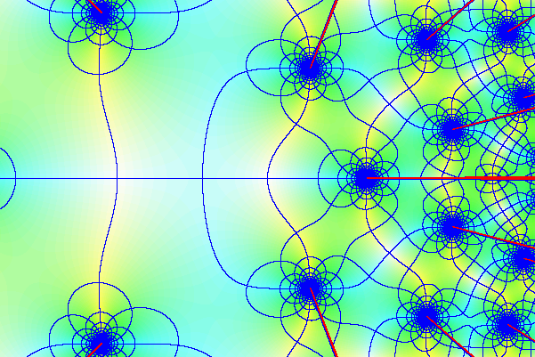
The Columbus program implements the approach of the present paper in the weaker setting of double precision complex numbers instead of effective complex numbers. We plan to describe this program in more details in a forthcoming paper and in particular the “radar algorithm” which is used to graphically represent analytic functions (see figure 1). It would be nice to adapt or reimplement the Columbus program so as to permit computations with effective complex numbers when desired.

The implementation of the Columbus program has also been instructive for understanding the complexity of our algorithms. For instance, the lower bound for the smallest zero in our algorithm for inversion can be extremely bad, as in the example

The problem here is that the effective radius of convergence is of the order of

, while the real radius is

. Consequently, the analytic continuation from

will take

steps instead of only

. In the Columbus program, this problem has been solved by using a numerical algorithm in order to determine the radius of convergence instead of the theoretically correct one. In some cases, this leads to an exponential speedup. Theoretically correct approaches for solving the problem are to compute the smallest zero of the denominator in an appropriate radius or to use transseries-like expansions. We plan to explain these approaches in more detail in a forthcoming paper.

Another trick which can be used in concrete implementations is to override the default evaluation method from section 2.5 by a more efficient one when possible, or to implement methods for the evaluation or computation of higher derivatives.

References

[BB85]: E. Bishop and D. Bridges. Foundations of constructive analysis. Die Grundlehren der mathematische Wissenschaften. Springer, Berlin, 1985.
[Car61]: H. Cartan. Théorie élémentaire des fonctions analytiques d'une et plusieurs variables. Hermann, 1961.
[CC90]: D.V. Chudnovsky and G.V. Chudnovsky. Computer algebra in the service of mathematical physics and number theory (computers in mathematics, stanford, ca, 1986). In Lect. Notes in Pure and Applied Math., volume 125, pages 109–232, New-York, 1990. Dekker.
[DL84]: J. Denef and L. Lipshitz. Power series solutions of algebraic differential equations. Math. Ann., 267:213–238, 1984.
[DL89]: J. Denef and L. Lipshitz. Decision problems for differential equations. The Journ. of Symb. Logic, 54(3):941–950, 1989.
[Kho91]: A. G. Khovanskii. Fewnomials. American Mathematical Society, Providence, RI, 1991.
[PG97]: A. Péladan-Germa. Tests effectifs de nullité dans des extensions d'anneaux différentiels. PhD thesis, Gage, École Polytechnique, Palaiseau, France, 1997.
[Ris75]: R.H. Risch. Algebraic properties of elementary functions in analysis. Amer. Journ. of Math., 4(101):743–759, 1975.
[Sha89]: J. Shackell. A differential-equations approach to functional equivalence. In Proc. ISSAC '89, pages 7–10, Portland, Oregon, A.C.M., New York, 1989. ACM Press.
[Sha93]: J. Shackell. Zero equivalence in function fields defined by differential equations. Proc. of the A.M.S., 336(1):151–172, 1993.
[SvdH01]: J.R. Shackell and J. van der Hoeven. Complexity bounds for zero-test algorithms. Technical Report 2001-63, Prépublications d'Orsay, 2001.
[vdH99]: J. van der Hoeven. Fast evaluation of holonomic functions. TCS, 210:199–215, 1999.
[vdH01a]: J. van der Hoeven. Fast evaluation of holonomic functions near and in singularities. JSC, 31:717–743, 2001.
[vdH01b]: J. van der Hoeven. Zero-testing, witness conjectures and differential diophantine approximation. Technical Report 2001-62, Prépublications d'Orsay, 2001.
[vdH02a]: Joris van der Hoeven. Columbus. http://www.math.u-psud.fr/~vdhoeven/Columbus/ Columbus.html, 2000–2002.
[vdH02b]: Joris van der Hoeven. A new zero-test for formal power series. In Teo Mora, editor, Proc. ISSAC '02, pages 117–122, Lille, France, July 2002.
[vdH02c]: Joris van der Hoeven. Relax, but don't be too lazy. JSC, 34:479–542, 2002.
[vdH03]: J. van der Hoeven. Majorants for formal power series. Technical Report 2003-15, Université Paris-Sud, 2003.
[vK75]: S. von Kowalevsky. Zur Theorie der partiellen Differentialgleichungen. J. Reine und Angew. Math., 80:1–32, 1875.

1Introduction

2Effective analytic functions

2.1Effective numbers and power series

2.2Effective germs

2.3Effective paths

2.4Effective analytic functions

2.5Analytic continuation along subdivided paths

3Operations on effective analytic functions

3.1Basic effective analytic functions

3.2The ring operations

3.3Differentiation and integration

3.4Inversion

3.5Exponentiation and logarithm

4Solving differential equations

4.1Linear differential equations

4.2Systems of algebraic differential equations

5Conclusion and final remarks

References