Fast Polynomial Multiplication over David Harvey School of Mathematics and Statistics University of New South Wales Sydney NSW 2052 Australia d.harvey@unsw.edu.au Joris van der Hoeven, Grégoire Lecerf Laboratoire d'informatique de l'École polytechnique LIX, UMR 7161 CNRS Campus de l'École polytechnique 1, rue Honoré d'Estienne d'Orves Bâtiment Alan Turing, CS35003 91120 Palaiseau, France {vdhoeven,lecerf}@lix.polytechnique.fr

Abstract

Can post-Schönhage–Strassen multiplication algorithms be competitive in practice for large input sizes? So far, the GMP library still outperforms all implementations of the recent, asymptotically more efficient algorithms for integer multiplication by Fürer, De–Kurur–Saha–Saptharishi, and ourselves. In this paper, we show how central ideas of our recent asymptotically fast algorithms turn out to be of practical interest for multiplication of polynomials over finite fields of characteristic two. Our Mathemagix implementation is based on the automatic generation of assembly codelets. It outperforms existing implementations in large degree, especially for polynomial matrix multiplication over finite fields.

Categories and Subject Descriptors

F.2.1 [Analysis of algorithms and problem complexity]: Numerical Algorithms and Problems—Computations in finite fields; G.4 [Mathematical software]: Algorithm design and analysis

General Terms

Algorithms, Theory

Keywords

Finite fields; Polynomial multiplication; Mathemagix

1.Introduction

Let denote the finite field with elements. In this article we are interested in multiplying polynomials in . This is a very basic and classical problem in complexity theory, with major applications to number theory, cryptography and error correcting codes.

1.1Motivation

Let denote the bit complexity of multiplying two polynomials of degree in . Until recently, the best asymptotic bound for this complexity was , using a triadic version [32] of the classical Schönhage–Strassen algorithm [33].

In [21], we improved this bound to , where The factor increases so slowly that it is impossible to observe the asymptotic behavior of our algorithm in practice. Despite this, the present paper demonstrates that some of the new techniques introduced in [20, 21] can indeed lead to more efficient implementations.

One of the main reasons behind the observed acceleration is that [21] contains a natural analogue for the three primes FFT approach to multiplying integers [30]. For a single multiplication, this kind of algorithm is more or less as efficient as the Schönhage–Strassen algorithm: the FFTs involve more expensive arithmetic, but the inner products are faster. On recent architectures, the three primes approach for integer multiplication generally has performance superior to that of Schönhage–Strassen due to its cache efficiency [25].

The compactness of the transformed representations also makes the three primes approach very useful for linear algebra. Accordingly, the implementation described in this paper is very efficient for matrix products over . This is beneficial for many applications such as half gcds, polynomial factorization, geometric error correcting codes, polynomial system solving, etc.

1.2Related work and our contributions

Nowadays the Schönhage–Strassen algorithm is widely used in practice for multiplying large integers [18] and polynomials [4, 19]. For integers, it was the asymptotically fastest known until Fürer's algorithm [11, 12] with cost , for input bit sizes , where is some constant (an optimized version [20] yields the explicit value ). However, no-one has yet demonstrated a practical implementation for sizes supported by current technology. The implementation of the modular variant proposed in [7] has even been discussed in detail in [28]: their conclusion is that the break-even point seems to be beyond astronomical sizes.

In [20, 21] we developed a unified alternative strategy for both integers and polynomials. Roughly speaking, products are performed via discrete Fourier transforms (DFTs) that are split into smaller ones. Small transforms then reduce to smaller products. When these smaller products are still large enough, the algorithm is used recursively. Since the input size decreases logarithmically between recursive calls, there is of course just one such recursive call in practice. Our implementation was guided by these ideas, but, in the end, only a few ingredients were retained. In fact, we do not recurse at all; we handle the smaller subproducts directly over with the Karatsuba algorithm.

For polynomials over finite fields, one key ingredient of [21] is the construction of suitable finite fields: we need the cardinality of their multiplicative groups to have sufficiently many small prime factors. A remarkable example is , outlined at the end of [21], for which we have:

Section 3 contains our first contribution: a detailed optimized implementation of DFTs over . We propose several original tricks to make it highly competitive on processors featuring carry-less products. For DFTs of small prime sizes we appeal to seminal techniques due to Rader [31] and Winograd [36]. Then the prime-factor algorithm, also called Good–Thomas [17, 35], is used in medium sizes, while the Cooley–Tukey algorithm [5] serves for large sizes.

In Section 4, we focus on other finite fields . When is a divisor of , we design efficient embeddings into , and compare to the use of Kronecker segmentation and padding. For values of up to , we propose a new algorithm to reduce computations to , in the vein of the three prime FFT technique. This constitutes our second contribution.

The practical performance of our implementation is reported in Section 5. We compare to the optimized reference library gf2x, developed by Brent, Gaudry, Thomé and Zimmermann [4], which assembles Karatsuba, Toom–Cook and the triadic Schönhage–Strassen algorithms with automatically tuned thresholds. The high performance of our implementation is of course a major outcome of this paper.

For detailed references on asymptotically fast algorithms to univariate polynomials over and some applications, we refer the reader to [4, 20, 21]. The present article does not formally rely on [21]. In the next section we recall and slightly adapt classical results, and present our implementation framework. Our use of codelets for small and moderate sizes of DFT is customary in other high performance software, such as FFTW3 and SPIRAL [10, 29].

2.Preliminaries

This section gathers classical building blocks used by our DFT algorithm. We also describe our implementation framework. If and are elements of a Euclidean domain, then and respectively represent the related quotient and remainder in the division of by , so that holds.

2.1Discrete Fourier transforms

Let be positive integers, let , , and . The -expansion of is the sequence of integers such that and

The -mirror, written , of relative to , is the integer defined by the following reverse expansion:

Let be a commutative field, and let be a primitive -th root of unity, which means that , and for all . The discrete Fourier transform (with respect to ) of an -tuple is the -tuple given by . In other words we have , where . For efficiency reasons, in this article, we compute the in the -mirror order, where corresponds to a certain ordering of the prime factors of , counted with multiplicities, that will be optimized later. We shall use the following notation:

Let , and let us split into and . We recall the Cooley–Tukey algorithm [5] in the present setting: it decomposes into and , where and .

Proposition 1. Algorithm 1 is correct.

Proof. Let be the successive values of the vector at the end of steps 1, 2, and 3. We have , , and . It follows that . The conclusion follows from , which implies .

Notice that the order of the output depends on , but not on . If the input vector is stored in a contiguous segment of memory, then the first step of Algorithm 1 may be seen as an matrix transposition, followed by in-place DFTs of size on contiguous data. Then the transposition is inverted. The constants in step 2 are often called twiddle factors. Transpositions affect the performance of the strided DFTs when input sizes do not fit in the last level cache memory of the processor.

For better locality, the multiplications by twiddle factors in step 2 are actually merged into step 3, and all the necessary primitive roots and fixed multiplicands (including the twiddle factors) are pre-computed once, and cached in memory. We finally notice that the inverse DFT can be computed straightforwardly by inverting Algorithm 1.

In addition to the Cooley–Tukey algorithm we shall also use the method attributed to Good and Thomas [17, 35], and that saves all the multiplications by the twiddle factors. First it requires the to be pairwise coprime, and second, input and output data must be re-indexed. The rest is identical to Algorithm 1—see [8], for instance, for complete formulas. With , the condition on the fails only when two are or . In such a case, it is sufficient to replace by a new vector where the two occurrences of (resp. of ) are replaced by (resp. by ), and to modify the re-indexing accordingly. In sizes 9 and 25, we build codelets upon the Cooley–Tukey formulas. A specific codelet for might further improve performance, but we did not implement this yet. We hardcoded the re-indexing into codelets, and we restrict to using the Good–Thomas algorithm up to sizes that fit into the cache memory. We shall discuss later the relative performance between these two DFT algoritms.

2.2Rader reduction

When the recurrence of the Cooley–Tukey algorithm ends with a DFT of prime size , then we may use Rader's algorithm [31] to reduce such a DFT to a cyclic polynomial product by a fixed multiplicand.

In fact, let , let be a generator of the multiplicative group of , and let be its modular inverse. We let and , and we compute . The coefficient of in equals . Consequently we have where is the permutation of defined by . In this way, the DFT of reduces to one cyclic product of size , by the fixed multiplicand .

Remark 2. Bluestein reduction [2] allows for the conversion of DFTs into cyclic products even when is not prime. In [21], this is crucially used for controlling the size of recursive DFTs. This suggests that Bluestein reduction might be useful in practice for DFTs of small composite orders, say . For DFTs over , this turns out to be wrong: so far, the strategies to be described in Section 3 are more efficient.

2.3Implementation framework

Throughout this article, we consider a platform equipped with an Intel(R) Core(TM) i7-4770 CPU at GHz and 8 GB of MHz DDR3 memory, which features AVX2 and CLMUL technologies (family number and model number 0x3C). The platform runs the Jessie GNU Debian operating system with a 64 bit Linux kernel version 3.14. Care has been taken to avoid CPU throttling and Turbo Boost issues while measuring timings. We compiled with GCC [15] version 4.9.2.

In order to efficiently and easily benefit from AVX and CLMUL instruction sets, we decided to implement the lowest level of our DFTs directly in assembly code. In fact there is no standard way to take full advantage of these technologies within languages such as C and C++, where current SIMD types are not even bona fide. It is true that programming via intrinsics [26] is a reasonable compromise, but there remain a certain number of technical pitfalls such as memory alignment, register allocation, and instruction latency management.

For our convenience we developed dynamic compilation features (also known as just in time compilation) from scratch, dedicated to high performance computing within Mathemagix (http://www.mathemagix.org). It is only used to tune assembly code for DFTs of orders a few thousands. Our implementation in the Runtime library partially supports the x86, SSE, and AVX instruction sets for the amd64 application binary interface—missing instructions can be added easily. This of course suits most personal computers and computation clusters.

The efficiency of an SSE or AVX instruction is not easy to determine. It depends on the types of its arguments, and is usually measured in terms of latency and throughput. In ideal conditions, the latency is the number of CPU clock cycles needed to make the result of an instruction available to another instruction; the reciprocal throughput, sometimes called issue latency, is the (fractional) number of cycles needed to actually perform the computation—for brevity, we drop “reciprocal”. For detailed definitions we refer the reader to [26], and also to [9] for useful additional comments.

In this article, we shall only use AVX-128 instructions, and 128-bit registers are denoted xmm0,…, xmm15 (our code is thus compatible with the previous generation of processors). A 128-bit register may be seen as a vector of two 64-bit integers, that are said to be packed in it. We provide unfamiliar readers with typical examples for our aforementioned processor, with cost estimates, and using the Intel syntax, where the destination is the first argument of instructions:

• vmovq loads/stores 64-bits integers from/to memory. vmovdqu loads/stores packed 64-bits integers not necessary aligned to 256-bit boundaries. vmovdqa is similar to vmovdqu when data is aligned on a 256-bit boundary; it is also used for moving data between registers. Latencies of these instructions are between 1 and 4, and throughputs vary between and .

• vpand, vpor, and vpxor respectively correspond to bitwise “and”, “or” and “xor” operations. Latencies are and throughputs are or .

• vpsllq and vpsrlq respectively perform left and right logical shifts on 64-bit packed integers, with latency 1 or , and throughput 1. We shall also use vpunpckhqdq xmm1, xmm2, xmm3/m128 to unpack and interleave in xmm1 the 64-bit integers from the high half of xmm2 and xmm3/m128, with latency and throughput 1. Here, xmm1, xmm2, and xmm3 do not mean that the instruction only acts on these specific registers: instead, the indices 1, 2, and 3 actually refer to argument positions. In addition, the notation xmm3/m128 means that the third argument may be either a register or an adress pointing to 128-bit data to be read from the memory.

• vpclmulqdq xmm1, xmm2, xmm3/m128, imm8 carry-less multiplies two 64-bit integers, selected from xmm2 and according to the constant integer imm8, and stores the result into xmm1. The value for imm8 means that the multiplicands are the 64-bit integers from the low half of xmm2 and xmm3/m128. Mathematically speaking, this corresponds to multiplying two polynomials in of degrees , which are packed into integers: such a polynomial is thus represented by a -bit integer, whose -th bit corresponds to the coefficient of degree . This instruction has latency 7 and throughput 2. This high latency constitutes an important issue when optimizing the assembly code. This will be discussed later.

3.DFTs over

In order to perform DFTs efficiently, we are interested in finite fields such that admits many small prime factors. This is typically the case [21] when admits many small prime factors itself. Our favorite example is , also because is only slightly smaller than the bit size of registers on modern architectures.

Using the eight smallest prime divisors of allows us to perform DFTs up to size , which is sufficiently large for most of the applications. We thus begin with building DFTs in size , , , , , , , , and then combine them using the Good–Thomas and Cooley–Tukey algorithms.

3.1Basic arithmetic in

The other key advantage of is the following defining polynomial . Elements of will thus be seen as polynomials in modulo .

For multiplying and in , we perform the product of the preimage polynomials, so that the preimage of may be obtained as follows

The remainder by may be performed efficiently by using bit shifts and bitwise xor. The final division by corresponds to a single conditional subtraction of .

In order to decrease the reduction cost, we allow an even more redundant representation satisfying the minimal requirement that data sizes are bits. If have degrees , then may be reduced in-place by , using the following macro, where xmm1 denotes any auxiliary register, and represents a register different from xmm1 that contains :

vpunpckhqdq xmm1, xmm0, xmm0
vpsllq xmm1, xmm1, 3
vpxor xmm0, xmm0, xmm1

In input contains the -bit packed polynomial, and its -bit reduction is stored in its low half in output. Let us mention from here that our implementation does not yet fully exploit vector instructions of the SIMD unit. In fact we only use the 64-bit low half of the -bit registers, except for DFTs of small orders as explained in the next paragraphs.

3.2DFTs of small prime orders

In size , it is classical that a DFT needs only one product and one reduction: . This strategy generalizes to larger as follows, via the Rader reduction of Section 2.2, that involves a product of the form

(1)

The coefficient of degree of satisfies:

(2)

This amounts to products, sums (even less if the are pre-computed), and reductions.

We handcrafted these formulas in registers for . Products are computed by vpclmulqdq. They are not reduced immediately. Instead we perform bitwise arithmetic on 128-bit registers, so that reductions to 64-bit integers are postponed to the end. The following table counts instructions of each type. Precomputed constants are mostly read from memory and not stored in registers. The last column cycles contains the number of CPU clock cycles, measured with the CPU instruction rdtsc, when running the DFT code in-place on contiguous data already present in the level 1 cache memory.

	clmul	shift	xor	move	cycles
3	1	2	7	6	19
5	10	8	22	10	37
7	21	12	45	14	58

For , these computations do not fit into the 16 registers, and using auxiliary memory introduces unwanted overhead. This is why we prefer to use the method described in the next subsection.

3.3DFTs of larger prime orders

For larger DFTs we still use the Rader reduction (1) but it is worth using Karatsuba's method instead of formula (2). Let , and let if is odd and 0 otherwise. We decompose , and , where have degrees . Then may be computed as , where , , and are obtained by the Karatsuba algorithm.

If is odd, then during the recursive calls for , we collect , for . Then we compute , so that the needed are obtained as .

During the recursive calls, reductions of products are discarded, and sums are performed over 128 bits. The total number of reductions at the end thus equals . We use these formulas for . For this approach leads to fewer products than with the previous method, but the number of sums and moves is higher, as reported in the following table:

	clmul	shift	xor	move	cycles
5	9	8	34	52	63
7	18	12	76	83	83
11	42	20	184	120	220
13	54	24	244	239	450
31	270	60	1300	971	2300
41	378	80	1798	1156	3000
61	810	120	3988	2927	7300

For readability only the two most significant figures are reported in column cycles. The measurements typically vary by up to about 10%. It might be possible to further improve these timings by polishing register allocation, decreasing temporary memory, reducing latency effects, or even by trying other strategies [1, 3].

3.4DFTs of composite orders

As long as the input data and the pre-computed constants fit into the level 3 cache of the processor (in our case, 8 MB), we may simply unfold Algorithm 1: we do not transpose-copy data in step 1, but rather implement DFT codelets of small prime orders, with suitable input and output strides. For instance, in size , we perform five in-place DFTs of order 3 with stride , namely on , then we multiply by those twiddle factors not equal to 1, and finally, we do three in-place DFTs of size and stride . In order to minimize the effect of the latency of vpclmulqdq, carry-less products by twiddle factors and reductions may be organized in groups of 8, so that the result of each product is available when arriving at its corresponding reduction instructions. More precisely, if rdi contains the current address to entries in , and rsi the current address to the twiddle factors, then 8 entry-wise products are performed as follows:

vmovq xmm0, [rdi+8*0]
vmovq xmm1, [rdi+8*1]
  …
vmovq xmm7, [rdi+8*7]
vpclmulqdq xmm0, xmm0, [rsi+8*0], 0
vpclmulqdq xmm1, xmm1, [rsi+8*1], 0
  …
vpclmulqdq xmm7, xmm7, [rsi+8*7], 0

Then the contents of xmm0,…,xmm7 are reduced in sequence modulo , and finally the results are stored into memory.

Up to sizes made from primes , we generated executable codes for the Cooley–Tukey algorithm, and measured timings for all the possible orderings . This revealed that increasing orders, namely , yield the best performances. In size , one transform takes CPU cycles, among which are spent in multiplications by twiddle factors. We implemented the Good–Thomas algorithm in the same way as for Cooley–Tukey, and concluded that it is always faster when data fit into the cache memory. When , this leads to only cycles for one transform, for which carry-less products contribute %.

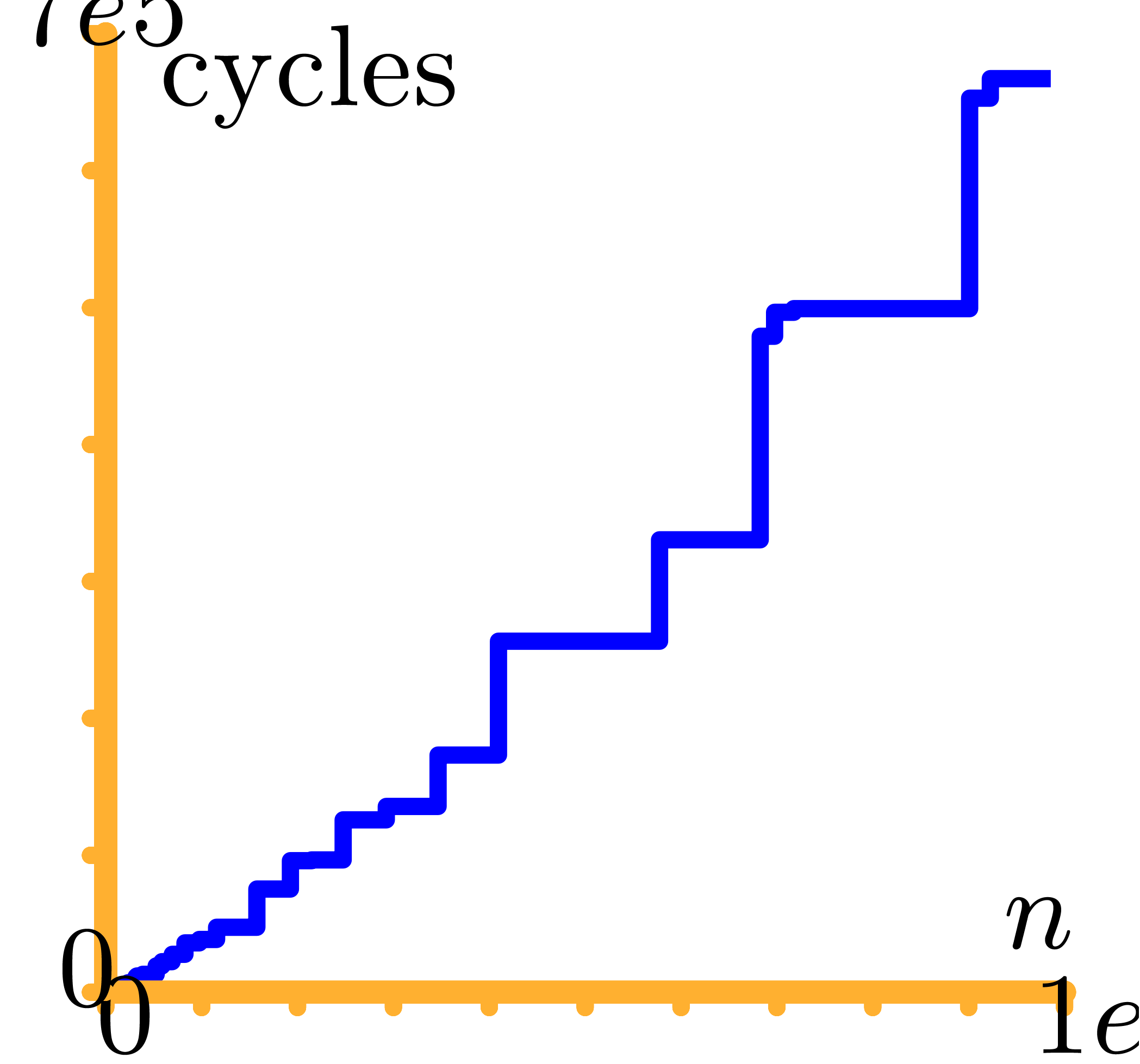
For each size , we then deduced the smallest DFT size , together with the best ordering, leading to the fastest calculation via the Good–Thomas algorithm. The graph in Figure 1 represents the number of CPU cycles in terms of obtained in this way. Thanks to the variety of prime orders, the staircase effect is softer than with the classical FFT.

For sizes larger than a few thousands, using internal DFTs of prime size with large strides is of course a bad idea in terms of memory management. The classical technique, going back to [16], and now known as the 4-step or 6-step FFT in the literature, consists in decomposing into such that and are of order of magnitude . In the context of Algorithm 1, with , and , we need to determine such that and are the closest to .

As previously mentioned, for large values of , step 1 of Algorithm 1 decomposes into the transposition of a matrix (in column representation), followed by in-place DFTs of size on contiguous data. Then the transposition is performed backward. In the classical case of the FFT, and are powers of two that satisfy or , and efficient cache-friendly and cache-oblivious solutions are known to transpose such matrices in-place with AVX2 instructions. Unfortunately, we were not able to do so in our present situation. Consequently we simply transpose rows in groups of 4 into a fixed temporary buffer of size . Then we may perform 4 DFTs of size on contiguous data, and finally transpose backward. The threshold for our 4-step DFTs has been estimated in the neighborhood of 7000.

4.Other ground fields

Usually, fast polynomial multiplication over is used as the basic building block for other fast polynomial arithmetic over finite fields in characteristic two. It is natural to ask whether we may use our fast multiplication over as the basic building block. Above all, this requires an efficient way to reduce multiplications in with to multiplications in . The optimal algorithms vary greatly with . In this section, we discuss various possible strategies. Timings are reported for some of them in the next section. In the following paragraphs, represent the two polynomials of degrees to be multiplied, and is the defining polynomial of over .

4.1Lifting and Kronecker segmentation

Case when . In order to multiply two packed polynomials in , we use standard Kronecker segmentation and cut the input polynomials into slices of 30 bits. More precisely, we set , and , so that and . The product then satisfies , where . We are thus led to multiply by in by reinterpreting as the generator of . In terms of the input size, this method admits a constant overhead factor of roughly . In fact, when considering algorithms with asymptotically softly linear cost, comparing relative input sizes gives a relevant approximation of the relative costs.

General strategies. It is well known that one can handle any value of by reduction to the case . Basically, is seen as , and a product in is lifted to one product in degree in , with coefficients of degrees in , followed by divisions by . Then, the Kronecker substitution [14, Chapter 8] reduces the computation of one such product in , said in bi-degree , to one product in in degree . In total, we obtain a general strategy to reduce one product in degree in to one product in in degree , plus bit operations. Roughly speaking, this approach increases input bit sizes by a factor at most in general, but only when .

Instead of Kronecker substitution, we may alternatively use classical evaluation/interpolation schemes [23, Section 2]. Informally speaking, a multiplication in in degree is still regarded as a multiplication of and in of bi-degrees , but we “specialize” the variable at sufficiently many “points” in a suitable ring , then perform products in of degrees , and finally we “interpolate” the coefficients of .

The classical Karatsuba transform is such a scheme. For instance, if then is sent to , which corresponds to the projective evaluation at . The size overhead of this reduction is , but its advantage to the preceding general strategy is the splitting of the initial product into smaller independent products. The Karatsuba transform can be iterated, and even Toom–Cook transforms of [3] might be used to handle small values of .

Another standard evaluation scheme concerns the case when is sufficiently large. Each coefficient of is “evaluated” via one DFT of size applied to the Kronecker segmentation of into slices of 30 bits seen in . Then we perform products in in degree , and “interpolate” the output coefficients by means of inverse DFTs. Asymptotically, the size overhead is again .

The rest of this section is devoted to other reduction strategies involving a size growth less than 4 in various particular cases.

4.2Field embedding

Case when When and , which corresponds to , we may embed into , by regarding as a field extension of . The input polynomials are now cut into slices of degrees with . The overhead of this method is asymptotically . If , then is odd, , and the overhead is . In particular it is only for .

Let be an irreducible factor of in , of degree . Elements of can thus be represented by polynomials of degrees in , modulo , via the following isomorphism

where represents the canonical preimage of in . Let be a polynomial of bi-degree representing an element of , obtained as a slice of or . The image can be obtained as . Consequently, if we pre-compute for all and , then deducing requires 59 sums in .

The number of sums may be decreased by using larger look-up tables. Let represent the basis for and , whatever the order is. Then all the for can be stored in 10 look-up tables of size 64, which allows to be computed using 9 sums. Of course the cost for reordering and packing bits of elements of must be taken into account, and sizes of look-up tables must be carefully adjusted in terms of . The details are omitted.

Conversely, let . We wish to compute . As for direct images of , we may pre-compute for all and reduce the computation of to sums in . Larger look-up tables can again help to reduce the number of sums.

Let us mention that the use of look-up tables cannot benefit from SIMD technologies. On the current platform this is not yet a problem: fully vectorized arithmetic in would also require SIMD versions of carry-less multiplication which are not available at present.

Case when . We may combine the previous strategies when is not coprime with . Let . We rewrite elements of into polynomials in of bi-degrees , and then use the Kronecker substitution to reduce to one product in in degree . For example, when , elements of may be represented by polynomials in . We are thus led to multiplying polynomials in in bi-degree , which yields an overhead of . Another favorable case is when , yielding an overhead of .

4.3Double-lifting

When , we may of course directly lift products in to products in of output degree in at most . The latter products may thus be computed as products in . This strategy has an overhead of , so it outperforms the general strategies for .

For , we lift products to and multiply in and . We then perform Chinese remaindering to deduce the product modulo .

Multiplying and in may be obtained as . In this way all relies on the same DFT routines over .

If has degree , with a power of , we decompose with and of degrees , then is obtained efficiently by the following induction:

			(3)

Chinese remaindering can also be done efficiently. Let be the inverse of modulo . Residues and then lift into modulo . Since , this formula involves only one carry-less product. Asymptotically, the overhead of this method is .

On our platform, formula (3) may be implemented in degree as follows. Assume that xmm0 contains , xmm1 contains , xmm2 contains 11110000…11110000, , and xmm5 is filled with 11…1100…00. Then, using xmm15 for input and output, we simply do

vpand xmm14, xmm15, xmm0
vpsrlq xmm14, xmm14, 1
vpxor xmm15, xmm14, xmm15
vpand xmm14, xmm15, xmm1
vpsrlq xmm14, xmm14, 2
vpxor xmm15, xmm14, xmm15
  …
vpand xmm14, xmm15, xmm5
vpsrlq xmm14, xmm14, 32
vpxor xmm15, xmm14, xmm15

4.4The Crandall–Fagin reduction

For “lucky” such that is irreducible over , multiplication in reduces to cyclic multiplication over of length . Using our adaptation [21] of Crandall–Fagin's algorithm [6], multiplying two polynomials of degrees in therefore reduces to one product in in degree , where is the first integer such that . The asymptotic overhead of this method is . This strategy generalizes to the case when divides , with .

For various , the polynomial factors into irreducible polynomials of degree . In that case, we may use the previous strategy to reduce products in to multiplications in , using different defining polynomials of . Asymptotically, the overhead reaches again , although working with different defining polynomials of probably involves another non trivial overhead in practice. Again, the strategy generalizes to the case when admits irreducible factors of degree with .

5.Timings

Our polynomial products are implemented in the Justinline library of Mathemagix. The source code is freely available from revision of our SVN server (http://gforge.inria.fr/projects/mmx/). Sources for DFTs over are in the file . Those for our polynomial products in are in polynomial_f2k_amd64_avx_clmul.mmx. Let us recall here that Mathemagix functions can also be easily exported to C++ [24].

We use version 1.1 of the gf2x library, tuned to our platform during installation. The top level function, named gf2x_mul, multiplies packed polynomials in , and makes use of the carry-less product instruction. Triadic variants of the Schönhage–Strassen algorithm start to be used from degree . gf2x can be used from versions of the NTL library [34], that uses Kronecker substitution to multiply in . Consequently, we do not need to compare to NTL. We also compare to FLINT 2.5.2, tuned according to §13 of the documentation.

5.1 and

Table 1 displays timings for multiplying polynomials of degrees in . The row “us” concerns the natural product via DFTs, the other row is the running time of gf2x_mul used to multiply polynomials in built from Kronecker substitution.

16 17 18 19 20 21 us gf2x

Table 1. Products in degree in , in milliseconds.

16 17 18 19 20 21 us gf2x flint

Table 2. Products in degree in , in milliseconds.

1 2 4 8 16 32 us gf2x 1300000

Table 3. Products of matrices over , in degree , in milliseconds.

16 17 18 19 20 21 us gf2x

Table 4. Products in degree in , in milliseconds.

16 17 18 19 20 21 us gf2x

Table 5. Products in degree in , in milliseconds.

In Table 2, we report on timings for multiplying polynomials of degrees in . The row “us” concerns our DFT based implementation via Kronecker segmentation, as recalled in Section 4.1. The row gf2x is the running time for the direct call to gf2x_mul. The row FLINT concerns the performance of the function nmod_poly_mul, which reduces to products in via Kronecker substitution. Since the packed representation is not implemented, we could not obtain timings until the end. This comparison is not intended to be fair, but rather to show unfamiliar readers why dedicated algorithms for may be worth it.

In both cases, our DFT based products turn out to be more efficient than the triadic version of the Schönhage–Strassen of gf2x, for large degrees. One major advantage of the DFT based approach concerns linear algebra. Instead of multiplying matrices over naively in time , we compute the DFTs and products of matrices over , in time . Matrix multiplication over is reduced to matrix multiplication over using similar techniques as in Section 4. Timings for matrices over , reported in Table 3, confirm the practical gain.

5.2 and

Table 4 displays timings for multiplying polynomials of degrees in . The row “us” concerns the double-lifting strategy of Section 4.3. The next row is the running time of gf2x_mul used to multiply polynomials in built from Kronecker substitution. As expected, timings for gf2x are similar to those of Table 1, and the overhead with respect to is close to . Overall, our implementation is about twice as fast than via gf2x.

Table 5 finally concerns our implementation of the strategy from Section 4.2 for products in degree in . As expected, timings are similar to those of Table 2 when input sizes are the same. We compare to the sole time needed by gf2x_mul used as follows: we rewrite the product in into a product in , which then reduces to products in in degrees thanks to Karatsuba's formula.

6.Conclusion

We are pleased to observe that key ideas from [20, 21] turn out to be of practical interest even for polynomials in of medium sizes. Besides Schönhage–Strassen-type algorithms, other strategies such as the additive Fourier transform have been developed for [13, 27], and it would be worth experimenting them carefully in practice.

Let us mention a few plans for future improvements. First, vectorizing our code should lead to a significant speed-up. However, in our implementation of multiplication in , we noticed that about the third of the time is spent in carry-less products. Since vpclmulqdq does not admit a genuine vectorized counterpart over 256-bit registers, we cannot hope for a speed-up of two by fully exploiting the AVX-256 mode. Then, the graph from Figure 1 can probably be further smoothed by adapting the truncated Fourier transform algorithm [22]. We are also investigating further accelerations of DFTs of prime orders in Section 3.3. For instance, for and , we might exploit the factorization in order to compute cyclic products using Chinese remaindering. In the longer run, we finally expect the approach in this paper to be generalizable to finite fields of higher characteristic

7.References