1.Introduction

Let be an effective ring of constants (i.e. the usual arithmetic operations , and can be carried out by algorithm). If has a primitive -th root of unity with , then the product of two polynomials with can be computed in time using the Fast Fourier Transform or FFT [CT65]. If does not admit a primitive -th root of unity, then one needs an additional overhead of in order to carry out the multiplication, by artificially adding new root of unity [SS71, CK91].

Besides the fact that the asymptotic complexity of the FFT involves a large constant factor, another classical drawback is that the complexity function admits important jumps at each power of two. These jumps can be reduced by using -th roots of unity for small . They can also be smoothened by decomposing -multiplications as -, - and -multiplications. However, these tricks are not very elegant, cumbersome to implement, and they do not allow to completely eliminate the jump problem.

In section 3, we present a new kind of “Truncated Fourier Transform” or TFT, which allows for the fast evaluation of a polynomial in any number of well-chosen roots of unity. This algorithm coincides with the usual FFT if is a power of two, but it behaves smoothly for intermediate values. In section 4, we also show that the inverse operation of interpolation can be carried out with the same complexity (modulo a few additional shifts).

The TFT permits to speed up the multiplication of univariate polynomials with a constant factor between and . In the case of multivariate polynomials, the repeated gain of such a constant factor leads to the gain of a non-trivial asymptotic factor. More precisely, assuming that admits sufficiently -th roots of unity, we will show in section 5 that the product of two multivariate polynomials can be computed in time , where and . The best previously known algorithm [CKL89], based on sparse polynomial multiplication, has time complexity .

In section 6 we finally give an algorithm for the multiplication of truncated multivariate power series. This algorithm, which has time complexity , again improves the best previously known algorithm [LS03] by a factor of . Moreover, both in the cases of multivariate polynomials and power series, we expect the corresponding constant factor to be better.

2.The Fast Fourier Transform

Let be an effective ring of constants, with and a primitive -th root of unity (i.e. ). The discrete Fast Fourier Transform (FFT) of an -tuple (with respect to ) is the -tuple with

In other words, , where denotes the polynomial .

The F.F.T can be computed efficiently using binary splitting: writing

we recursively compute the Fourier transforms of and

Then we have

This algorithm requires multiplications with powers of and additions (or subtractions).

In practice, it is most efficient to implement an in-place variant of the above algorithm. We will denote by the bitwise mirror of at length (for instance, and ). At step , we start with the vector

At step , we set

(1)

for all and , where . Using induction over , it can easily be seen that

for all and . In particular,

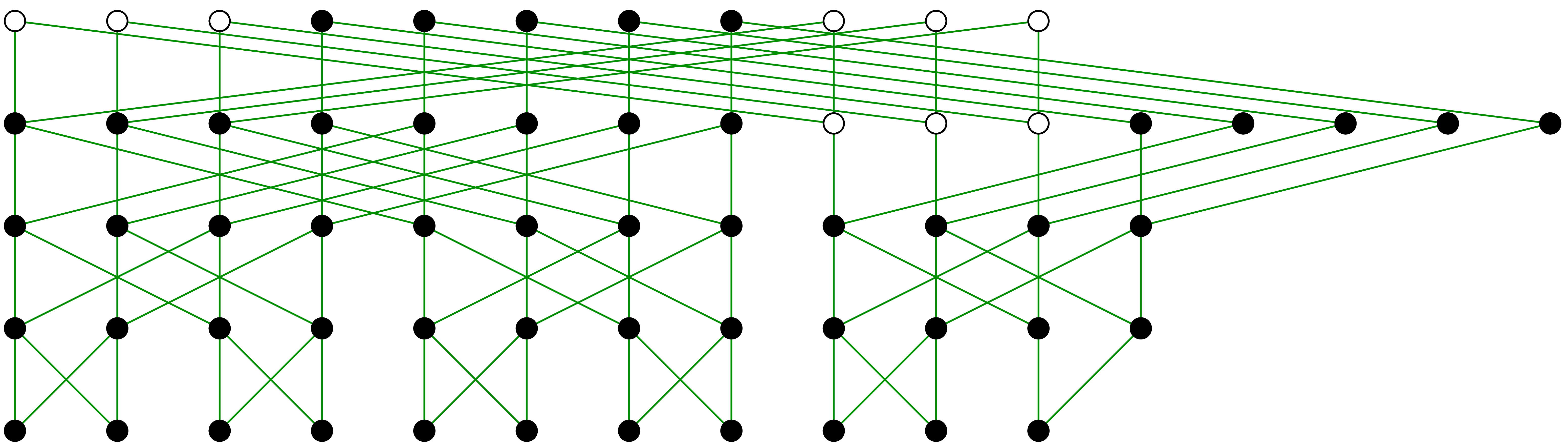
for all . This algorithm of “repeated crossings” is illustrated in figure 1.

Figure 1. Schematic representation of a Fast Fourier Transform for . The black dots correspond to the , the upper row being and the lower row .

A classical application of the FFT is the multiplication of polynomials and . Assuming that , we first evaluate and in using the FFT:

We next compute the evaluations of at . We finally have to recover from these values using the inverse FFT. But the inverse FFT with respect to is nothing else as times the direct FFT with respect to . Indeed, for all and all , we have

(2)

since

whenever . This yields a multiplication algorithm of time complexity in , when assuming that admits enough primitive -th roots of unity. In the case that does not, then new roots of unity can be added artificially [SS71, CK91, vdH02] so as to yield an algorithm of time complexity .

3.The Truncated Fourier Transform

The algorithm from the previous section has the disadvantage that needs to be a power of two. If we want to multiply two polynomials such that , then we need to carry out the FFT at precision , thereby losing a factor of . This factor can be reduced using several tricks. For instance, one may decompose the -product into an product, an -product and an -product. This is efficient for small , but not very good if . In the latter case, one may also use an FFT at precision , by using -matrices at one step of the FFT computation. However, all these tricks of the trade require a large amount of hacking and one always continues to lose a non-trivial factor between and .

The idea behind the Truncated Fourier Transform is to provide an efficient algorithm for the evaluation of polynomials in any number of distinct points. Moreover, the inverse operation of interpolation can be carried out with the same complexity (modulo a few additional shifts). This technique will eliminate the “jumps” in the complexity of FFT multiplication.

So let , (usually, ) and let be a primitive -th root of unity. Given an -tuple , we will evaluate the corresponding polynomial in . We call the Truncated Fourier Transform (TFT) of . Now consider the completion of the -tuple into an -tuple . When using the in-place algorithm from the previous section in order to compute , we claim that many of the computations of the can actually be skipped (see figure 2). Indeed, at stage , it suffices to compute the vector . Besides , we therefore compute at most additional values. In total, we therefore compute at most values . This proves the following result:

Figure 2. Schematic representation of a TFT for and .

Remark 2. Assume that admits a privileged primitive -th root of unity for every , such that for all . Then the TFT of an -tuple w.r.t. with does not depend on the choice of . We call the TFT of w.r.t. the privileged sequence of roots of unity.

Remark 3. Since the only operations we need for computing the TFT are additions, subtractions and multiplications by powers of , the algorithm naturally combines with Schönhage-Strassen's algorithm when is a symbolically added root of unity.

Remark 4. If , then the TFT of can be computed using ring operations using a similar algorithm as above. More generally, this allows the rapid transformation of “unions of segments”.

4.

Inverting the Truncated Fourier Transform

Unfortunately, the inverse TFT cannot be computed using a similar formula as (2). Indeed, starting with the , we need to compute an increasing number of when decreases. Therefore we will rather invert the algorithm which computes the TFT, but with this difference that we will sometimes need with in order to compute . We will use the fact that whenever one value among , and one value among , are known in the cross relation (1), then we can deduce the others from them using one multiplication by a power of and two “shifted” additions or subtractions (i.e. the results may have to be divided by ).

More precisely, let us denote and at each stage . We use a recursive algorithm which takes the values and on input, and which computes . If , then we have nothing to do. Otherwise, we distinguish two cases:

• If , then we first compute from using repeated crossings. We next deduce and from and for all . Invoking our algorithm recursively, we now obtain . We finally compute and from and for .

• If , then we first compute from and for . Invoking our algorithm recursively, we next compute . We finally deduce from and for all .

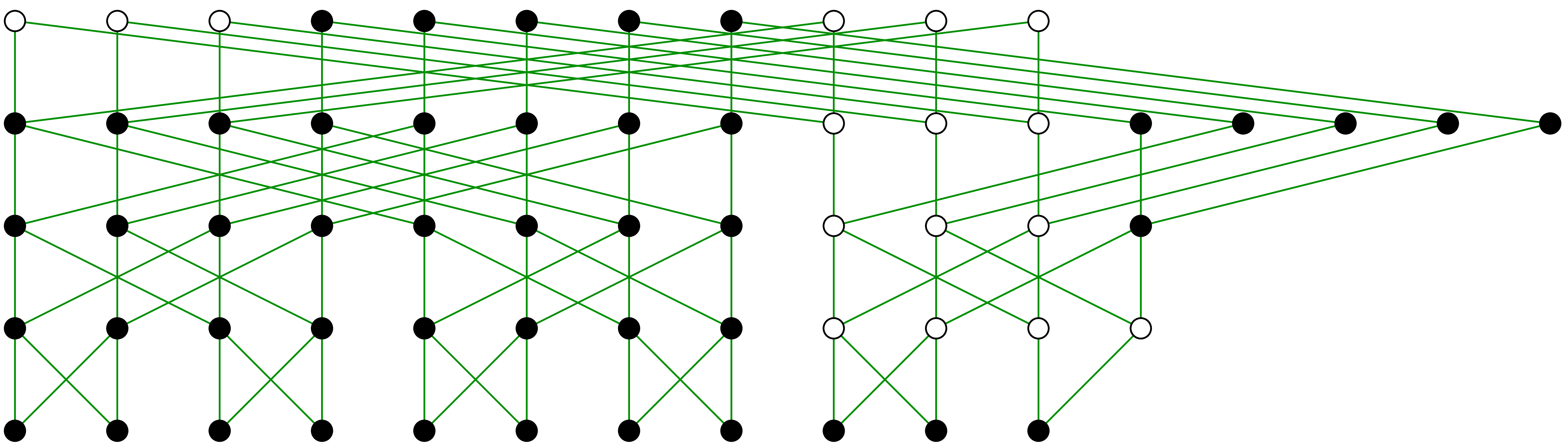
The two cases are illustrated in figures 3 resp. 4. Since , the application of our algorithm for computes the inverse TFT. We notice that the values with are computed in decreasing order (for ) and the values with in increasing order. In other words, the algorithm may be designed in such a way to remain in place. We have proved:

Figure 3. Schematic representation of the recursive computation of the inverse TFT for , . The different images show the progression of the known values (the black dots) during the different computations at stage . Since , we fall into the first case of our algorithm and the recursive invocation of the algorithm is done between the third and the fourth image.

Figure 4. Schematic representation of the recursive computation of the inverse TFT for , at stage . Since and , we now fall into the second case of our algorithm and the recursive invocation of the algorithm is done between the third and the fourth image.

Remark 6. Besides shifted additions, subtractions or multiplications by powers of , the algorithm essentially computes inverse FFT-transforms of sizes with . Using (2), it is therefore possible to replace all but shifted additions and subtractions by normal additions and subtractions.

5.Multiplying multivariate polynomials

Let be a ring with a privileged sequence of roots of unity (see remark 2). Given a non-zero multivariate polynomial

in variables, we define the total degree of by

We let . Now let be such that . In this section we present an algorithm to compute , which has a good complexity in terms of the number

of expected coefficients of . When computing using the classical FFT with respect to each of the variables , we need a time which is much bigger than , in general. When using multiplication of sparse polynomials [CKL89], we need a time with a non-trivial constant factor. Our algorithm is based on the TFT w.r.t. all variables and we will show that it has a complexity .

Given with , the TFT of with respect to one variable at order is defined by

where . We recall that the result does not depend on the choice of . The TFT with respect to all variables at order is defined by

where (see figure 5). We have

Given with , we will use the formula

in order to compute the product .

Figure 5. Illustration of the TFT in two variables ().

In order to compute , say for , we compute the TFT of with for all with (if , then the TFT of is given by itself, so we have nothing to do). One such computation takes a time for some universal constant , by using the TFT w.r.t. with minimal (so may vary as a function of , but not ). The computation of therefore takes a time with

Dividing by , we obtain

			(3)

If , then the summand rapidly deceases when , so that

Consequently, and even for fixed . If , then for and , Stirling's formula yields

It follows that only the first terms in (3) contribute to the asymptotic behaviour of , so that

Again, we find that . We have proved:

6.Multiplying multivariate power series

Since power series have infinitely many terms, implementing an operation on power series really corresponds to implementing the operation for polynomial approximations at all degrees. As usual, multiplication is a particularly important operation. Given with and , we will show how to compute the truncated product of and .

The first idea [LS03] is to use homogeneous coordinates instead of the usual ones:

This transformation takes no time since it corresponds to some re-indexing. We next compute the TFTs and in at order :

We next compute the truncated products of the obtained polynomials and . After transforming the results of these multiplication back using

we obtain the truncated product of and by

The total computation time is bounded by . Using the fact that , we have proved the following theorem:

Remark 9. In practice, if the coefficients have different growths in , then it may be useful to consider truncations along more general degrees of the form

The “slicing technique” from section 6.3.5 in [vdH02] may then be used in order to obtain complexity bounds of the same type.

Remark 10. Using remark 4, the polynomial and truncated multiplication algorithms can be used in combination with the strategy of relaxed evaluation [vdH97, vdH02, vdH03b] for solving partial differential equations in multivariate power series with an additional overhead of . A recent technique [vdH03a] allows to reduce this overhead even further and it would be interesting to study more precisely what happens in the multivariate case.

7.Final notes

The author would like to thank the first referee for his enthusiastic and helpful comments. This referee also implemented the algorithms from sections 3 and 4 and he reports a behaviour which is close to the expected one. In response to some other comments and suggestions, we conclude with the following remarks:

• The results of the paper may be generalized to characteristic 2 and general rings along similar lines as in [CK91]. The crucial remark is that, if and

  

  then, for all , we may compute in terms of by using only additions, subtractions, multiplications by and divisions by .

• Theorem 1 in [CKL89] implies theorem 7 with replaced by . The technique from [CKL89] is actually more general: let and assume that we know

  

  If and are not “extraordinarily sparse”, then may be computed in time . It would be interesting to prove something similar in our context, so as to examine to which extent we need the density hypothesis. Using remark 4 in a recursive way, we expect that there exists an algorithm of complexity , for a suitable definition of .

• The terminology of privileged sequences may seem to be an overkill. Indeed, in practice, we rather need a sufficiently large root of unity in order to carry out a given computation. Nevertheless, from a theoretical point of view, this paper suggests that it may be interesting to study “fractal FFT-transforms” of power series with convergence radius with respect to a privileged sequence .

• Two referees pointed us to the recent on-line paper [Ber] which also contains the idea of evaluating in powers of in order to multiply polynomials with .

Bibliography