In the last years, several asymptotic expansion algorithms have appeared, which have the property that they can deal with very general types of singularities, such as singularities arising in the study of algebraic differential equations. However, attention has been restricted so far to functions with “strongly monotonic” asymptotic behaviour: formally speaking, the functions lie in a common Hardy field, or, alternatively, they are determined by transseries. In this article, we make a first step towards the treatment of functions involving oscillatory behaviour. More precisely, let be an algebraic function defined on , let be exp-log functions at infinity in , and let We give a method to compute . Moreover, the techniques we use are stronger than this result might suggest, and we outline further applications. Keywords: Asymptotic expansion, exp-log function, oscillating function, Diophantine approximation, algorithm A.M.S. subject classification: 03H05, 11J25, 11J61, 11J71, 11K06, 11K36, 12L15, 14P10, 14P15, 26A03, 26A09, 26A12, 26A48, 26E30, 28D99, 41A58, 41A60, 68Q25

1.Introduction

In the last years, several asymptotic expansion algorithms have appeared [Sha90, Sha91, GG92, RSSH96, Hoe96a]. These algorithms are have the property that they can deal with very general types of singularities, such as singularities arising in the study of certain algebraic differential equations. However, attention has been restricted so far to functions with “strongly monotonic” asymptotic behaviour. This means that the functions lie in a common Hardy field, or, alternatively, that they are determined by transseries. In this article, we make a first step to the treatment of functions involving oscillatory behaviour. We also notice that Grigoriev obtained some very interesting related results in [Gri94, Gri95] although his more probabilistic point of view is different (even complementary) from ours.

The structure of this paper is as follows: in section 2, we recall a classical density theorem for linear curves on the -dimensional torus (see for example [Kok36, KN74]). In section 3, this theorem is generalized to more general classes of curves on the torus.

In section 4, we study exp-log functions at infinity: an exp-log function is a function which is built up from the rationals and , using the field operations, exponentiation and logarithm. An exp-log function at infinity is an exp-log function which is defined in a neighbourhood of infinity. We present a more compact version of an expansion algorithm of exp-log functions at infinity, originally due to Shackell [Sha91] (see also [RSSH96]). For this, we assume the existence of an oracle for deciding whether an exp-log function is zero in a neighbourhood of infinity. This problem has been reduced to the corresponding problem for exp-log constants in [Hoe96b, Hoe96a]. A solution to the constant problem was given by Richardson in [Ric94], modulo Schanuel's conjecture:

In section 5, we are given an algebraic function defined on , and exp-log functions at infinity in . We show how to compute

In section 5, we will assume the existence of an oracle for checking the -linear dependence of exp-log constants. Actually, Richardson's algorithm can easily be adapted to yield an algorithm for doing this modulo Schanuel's conjecture.

2.A density theorem on the -dimensional torus

Let be -linearly independent numbers: we will use vector notation, and denote the vector by . In this section, we prove that the image of , from in the -dimensional torus is dense. Notice that we use the same notation for and its class modulo . Moreover, we show that the “density” of the image is uniform is a sense that will be made precise. The following theorem is classical:

Now let be a measurable subset of , and let be some interval of . Denoting the Lebesgue measure by , we define

(1)

Let us also denote by the Euclidean distance on . Let , resp. denote the shift operator on (resp. or ): and . The following are immediate consequences of the definition of :

It will be convenient to adopt some conventions for intervals (resp. or ) whose lengths tend to infinity: we say that a property holds uniformly in , if the property holds uniformly in :

We say that holds for all sufficiently close to infinity, if holds for all sufficiently large .

The next theorem is also classical, but for convenience of the reader we present a proof, since similar techniques will be used in the next section:

Theorem 4. (Bohr, Sierpiński, Weyl) Let be -linearly independent real numbers and let be given by (1). Let

be an -dimensional block, with for all . Then

uniformly in .

Proof. The theorem trivially holds if and for all but one . Hence, it suffices to prove the theorem when the 's and the 's are rational numbers. Indeed, let be rational numbers with , and denote . Then for sufficiently large, uniformly in .

Because of Proposition 3(a) and (b), it suffices to prove the theorem for fixed and for all

with . We remark that , so that .

Now let . For each , we can find , with , by Proposition 2. Consequently, we have , where denotes the symmetric difference of and . Hence, , for each with . Using Proposition 3, we can now estimate

Taking , for any and , we get

Hence , for sufficiently large , uniformly in . This completes our proof.

3.A more general density theorem

In this section we will obtain a more general uniform density theorem on the torus, when the application from section 2 is replaced by a non linear mapping, which satisfies suitable regularity conditions. Before coming to this generalization, we will need some definitions and lemmas. We say that a function defined in a neighbourhood of infinity is steadily dominated by , if has a continuous second derivative, tends to infinity, decreases strictly towards zero, and tends to zero. We remark that such functions admit functional inverses in a neighbourhood of infinity.

More generally, we say that if and are functions in a neighbourhood of infinity, such that is invertible, then is steadily dominated by , if is steadily dominated by . In this case, we write . It is easily verified that if and , then , so that is transitive. We also remark that if and if is a function, which has a continuous second derivative and tends to infinity, then . We finally have the following property of steady domination:

Proof. Let be such that , for all . We have , for some between and . If is positive, then , and we are done. In the other case, we have , whence .

Now let be a measurable subset of . For each interval , we define:

We say that admits an asymptotic density if

uniformly in , for sufficiently close to infinity. More generally, if is steadily dominated by , then we say that admits -asymptotic density if

uniformly in , for sufficiently close to infinity.

Proof. Let . Let be such that , whenever . Let with and subdivide in parts of equal length :

with for . Then we have

By Lemma 5, for all sufficiently large , we have , for all with . Hence,

and we have a similar estimation, when replacing by . Consequently,

This completes our proof.

Let be continuous functions defined in a neighbourhood of infinity, which strictly increase towards infinity. Let () be such that are -linearly independent for each . Now consider the curve

on (), which is defined for sufficiently large . By analogy with the preceding section, we define

(2)

for intervals sufficiently close to infinity, and measurable subsets of .

Theorem 7. Let and be given as above and let

be an -dimensional block. Then

uniformly, for intervals sufficiently close to infinity.

Proof. We proceed by induction over . If , we have nothing to prove. As before, it suffices to prove the theorem for multidimensional blocks , with and , where . We denote by resp. the projections of on resp. , when considering as the product of and . Without loss of generality, we may assume that .

Given a subset of or and its frontier , we denote for any

Let . If , then for all with , where . Hence, for sufficiently close to infinity,

Therefore, Theorem 4 implies that for sufficiently close to infinity

(3)

and (using that )

(4)

Now is a finite union of intervals, say

where have length at least , and where and have length at most .

By the induction hypothesis, we have

uniformly, for sufficiently close to infinity. Using Lemma 6 for , this gives us

uniformly, for sufficiently close to infinity. In particular, we have

for all sufficiently close to infinity, with . Thus, choosing sufficiently close to infinity, we have

for all .

Taking , and using (3) and (4), this gives us

This completes the proof.

4.Expansions of exp-log functions at infinity

Let denote the field of germs at infinity of exp-log functions and the subfield of exp-log constants. Elements of can be represented by exp-log expressions — i.e. finite trees whose internal nodes are labeled by or , and whose leaves are labeled by or rational numbers. The set of exp-log expressions which can be evaluated in a neighbourhood of infinity is denoted by . We have a natural projection from onto . We make the assumption that we have at our disposal an oracle which can decide whether a given exp-log expression in is zero in a neighbourhood of infinity. In view of [Hoe96b, Hoe96a] it actually suffices to assume the existence of an oracle to decide whether a given exp-log constant is zero.

4.1.Grid-based series

Let us first recall some basic concepts. An effective asymptotic basis is an ordered finite set of positive infinitesimal exp-log expressions in , such that (i.e. ) for . For instance, the set is an effective asymptotic basis. An effective asymptotic basis generates an effective asymptotic scale, namely the set of all products of powers of the 's, with the 's in . Elements of are also called monomials.

Given an effective asymptotic basis , let denote the set of expressions which are built up from and the operations , resp. , for infinitesimal . We observe that can be expanded as a series in with coefficients in . Moreover, these coefficients can recursively be expanded in :

The exp-log expressions of the form are called iterated coefficients of . In particular, the iterated coefficients of the form are exp-log constants.

The above expansions of have an important property [Hoe96a]: the support of as a series in is included in a set of the form , where the 's and are constants in — we say that is a grid-based series. From this property, it follows that the support of is well-ordered.

Another important property of the expansion of in and the expansions of its iterated coefficients is that they can be computed automatically. By this we mean that for each integer , we can compute the first terms of the expansion of and so can we for its iterated coefficients. In particular, we can compute the sign of , test whether is infinitesimal, etc.

For the computation of the expansions of in , we use the usual Taylor series formulas. In the case of division , we compute the first term of and then use the formula , where . The only problem when applying these formulas is that we have to avoid indefinite cancelation: note that indefinite cancelation only occurs if after having computed the first terms of the expansion, is actually equal to the sum of these terms. But this can be tested using the oracle, and we stop the expansion in this case.

4.2.Automatic expansions of exp-log expressions

The asymptotic expansion algorithm takes an exp-log expression on input, computes a suitable effective asymptotic basis and rewrites into an element of . The main idea of the algorithm lies in imposing some suitable conditions on : we say that a linearly ordered set is an effective normal basis if

NB1

is an effective asymptotic basis.

NB2

for all , where .

NB+

for some , where .

Such a basis is constructed gradually during the algorithm — i.e. is a global variable in which we insert new elements during the execution of the algorithm, while maintaining the property that is an effective normal basis. We also say that is a dynamic effective normal basis. Let us now explicitly give the algorithm, using a PASCAL-like notation:

Algorithm . The algorithm takes an exp-log expression on input and rewrites it into a grid-based series in , where the global variable contains an effective normal basis which is initialized by .

case : return

case : return

case , where :

if and then error “division by zero”

return

case :

Denote .

if then error “invalid logarithm”

Rewrite , with infinitesimal in and .

if then

return

case :

Denote .

if then return , where

if then

return

Let be such that .

return

Let us comment the algorithm. The first three cases do not need explanation. In the case , the fact that is an effective normal basis is used at the end: is indeed an expression in . The expansion of the exponential of a bounded series is done by a straightforward Taylor series expansion. If is unbounded, then we test whether is asymptotic to the logarithm of an element in — i.e. we test whether is a non zero finite number for some . If this is so, then and is expanded recursively. We remark that no infinite loop can arise from this, because successive values of in such a loop would be asymptotic to the logarithms of smaller and smaller elements of , while remains unchanged. Finally, if is not asymptotic to the logarithm of an element in , then has to be extended with an element of the order of growth of . The decomposition is computed in order to ensure that remains an effective normal basis.

5.On the automatic computation of limsups

In this section we show how Theorem 7 can be applied to compute limsups (or liminfs) of certain bounded functions, involving trigonometric functions. The idea is based on the following consequence of Theorem 7.

Theorem 8. Let be exp-log functions at infinity. Let () be such that are -linearly independent for each . Denote and . Let be a continuous function from into and let

Then

Proof. We first notice that we will be able to apply Theorem 7 on our input data: by a well known theorem, which goes back to Hardy [Har11], the germs at infinity of lie in a common Hardy field. Consequently, , and are strictly increasing in a suitable neighbourhood of infinity.

The mapping is defined in a neighbourhood of infinity, and can be factored , with

and

where and are both continuous. Since is compact, there exists a point in which attains its maximum. Let . There exists a neighbourhood of , such that , for any in . By Theorem 7, there exist , with as close to infinity as we wish. For such , we have .

We now turn to the computation of this limit.

Proof. Using the identity , we may always assume without loss of generality, that the 's are all positive. Now the algorithm consists of the following steps:

Step 1. Compute a common effective normal basis for , using the algorithm from section 4. Order the 's w.r.t. ; that is, or , whenever .

Step 2. Simultaneously modify the 's and the algebraic function in the 's, until we either have , or , for some , whenever . As long as this is not the case, we take maximal, such that the above does not hold, and do the following:

First compute the limit of . Next insert and into the set of 's and remove . The new expression for is obtained by replacing each by .

Step 3. Compute exp-log functions , and constants (), such that each can be written as , for some and . Replacing by its limit for each bounded , we reduce the general case to the case when .

Step 4. This step consists in making the 's -linearly independent for each fixed . Whenever there exists a non trivial -linear relation between the 's (for fixed ), we may assume without loss of generality that this relation is given by

for in and . As long as we can find such a relation, we do the following:

For all , replace by and by in the expression for . Next, replace by in the expression for .

Step 5. By Theorem 8, the limsup of is the maximum of on , where . To compute this maximum, we determine the set of zeros of the gradient of on . Then is constant on each connected component and the maximum of these constant values yields . To compute the zero set of the gradient of and its connected components, one may for instance use cylindrical decomposition (see [Col75]). Of course, other algorithms from effective real algebraic geometry can be used instead.

The correctness of our algorithm is clear. The termination of the loop in step 2 follows from the fact that the new is asymptotically smaller then , so that either the -class of strictly decreases, or the number of 's with , but not for some . The number of -classes which can be attained is bounded by the initial value of .

Corollary 10.

Let be exp-log functions at infinity and be an algebraic function in variables, defined on . Assume that we have an oracle to test the -linear dependence of exp-log constants. Then there exists an algorithm to compute the limsup of .

Example 11. Consider the function

The first step consists in expanding , , and . All these functions have the same -class, but they are not all homothetic. Therefore, some rewriting needs to be done. First, , and we rewrite

which corresponds to the rewriting

if we consider real and imaginary parts. Similarly, we rewrite

which corresponds to the rewriting

In step 4, no -linear relations are found, so that we have to determine the maximal value of

(5)

on . Here we have abbreviated (hence is the set of points with ). The maximum of is attained for . We deduce that

Similarly, exploiting the symmetry of (5), we have

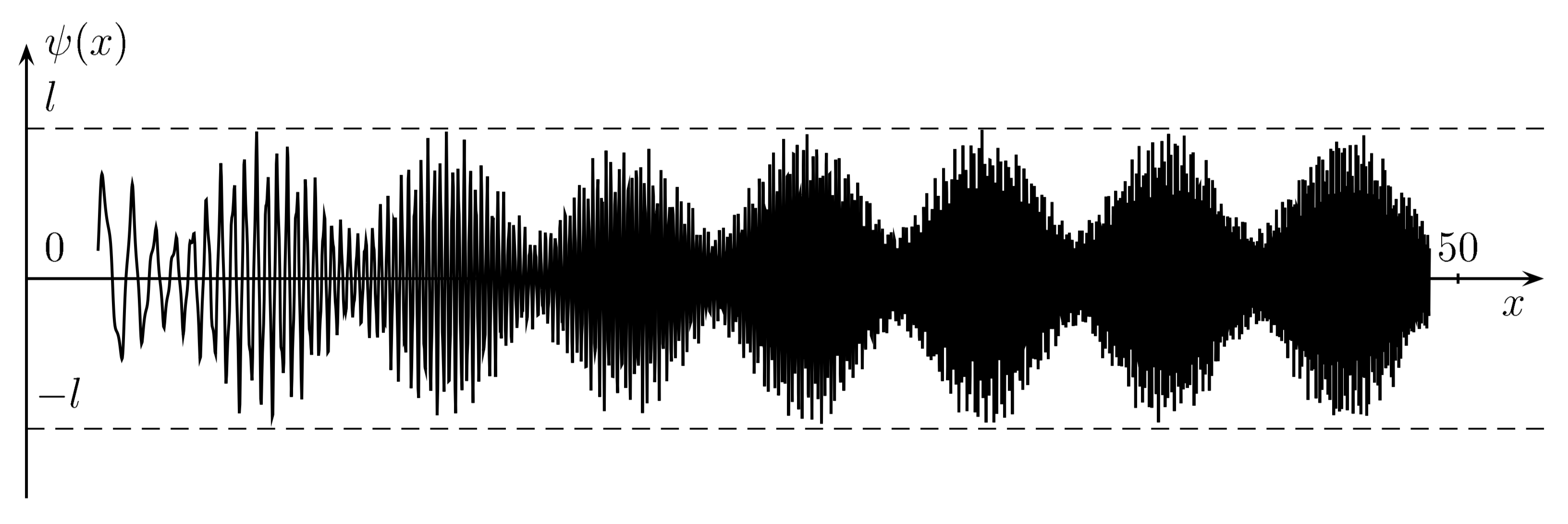Figure 1. Plot of the function from Example 11.

6.Conclusion

We have shown how to compute limsups of certain functions involving trigonometric functions, exponentiation and logarithm. Actually, the techniques we have used are far more general than Theorem 9 might suggest. Let us now briefly mention some generalizations. For more details, we refer to [Hoe96a].

In Theorem 9, the crucial property of the functions is that they are strongly monotonic and that we have an asymptotic expansion algorithm for them. Consequently, more general functions than exp-log functions can be taken instead, like Liouvillian functions, functions which are determined by systems of real exp-log equations in several variables, etc.

The crucial property of the function is that it belongs to a class for which a cylindrical decomposition algorithm exists. Again, more general classes of functions can be considered. In particular, modulo suitable oracles, one can consider the class of solutions to real exp-log systems in several variables.

Our techniques can also be used to compute automatic asymptotic expansions of sin-exp-log functions at infinity of trigonometric depth one (i.e. without nested sines). However, some difficult number theoretical phenomena may occur in this case, as the following example illustrates:

This asymptotic inequality follows from the number theoretical properties of . In general, such inequalities are very hard to obtain (if decidable at all!): a systematic way to obtain them would in particular yield solutions to deep unsolved problems in the field of Diophantine approximation (for a nice survey, see [Lan71]).

Nevertheless, we notice that the above example is “degenerate” in the sense that is precisely equal to the limsup of . In the generic case, a complete asymptotic expansion for sin-exp-log functions at infinity of trigonometric depth one does exist. In the degenerate case, we need assume the existence of a suitable oracle for Diophantine questions.

Bibliography