4.3The field of grid-based transseries in |
87 |
|
Foreword |
XI |
Introduction |
1 |
The field with no escape |
1 |
Historical perspectives |
3 |
Outline of the contents |
7 |
Notations |
10 |
1Orderings |
11 |
1.1Quasi-orderings |
12 |
1.2Ordinal numbers |
15 |
1.3Well-quasi-orderings |
17 |
1.4Kruskal's theorem |
19 |
1.5Ordered structures |
22 |
1.6Asymptotic relations |
25 |
1.7Hahn spaces |
29 |
1.8Groups and rings with generalized powers |
30 |
2Grid-based series |
33 |
2.1Grid-based sets |
34 |
2.2Grid-based series |
36 |
2.3Asymptotic relations |
40 |
2.3.1Dominance and neglection relations |
40 |
2.3.2Flatness relations |
42 |
2.3.3Truncations |
42 |
2.4Strong linear algebra |
44 |
2.4.1Set-like notations for families |
44 |
2.4.2Infinitary operators |
45 |
2.4.3Strong abelian groups |
46 |
2.4.4Other strong structures |
47 |
2.5Grid-based summation |
48 |
2.5.1Ultra-strong grid-based algebras |
48 |
2.5.2Properties of grid-based summation |
49 |
2.5.3Extension by strong linearity |
50 |
2.6Asymptotic scales |
53 |
3The Newton polygon method |
57 |
3.1The method illustrated by examples |
58 |
3.1.1The Newton polygon and its slopes |
58 |
3.1.2Equations with asymptotic constraints and refinements |
59 |
3.1.3Almost double roots |
62 |
3.2The implicit series theorem |
63 |
3.3The Newton polygon method |
65 |
3.3.1Newton polynomials and Newton degree |
65 |
3.3.2Decrease of the Newton degree during refinements |
66 |
3.3.3Resolution of asymptotic polynomial equations |
67 |
3.4Cartesian representations |
69 |
3.4.1Cartesian representations |
69 |
3.4.2Inserting new infinitesimal monomials |
71 |
3.5Local communities |
71 |
3.5.1Cartesian communities |
72 |
3.5.2Local communities |
72 |
3.5.3Faithful Cartesian representations |
73 |
3.5.4Applications of faithful Cartesian representations |
74 |
3.5.5The Newton polygon method revisited |
75 |
4Transseries |
79 |
4.1Totally ordered exp-log fields |
80 |
4.2Fields of grid-based transseries |
84 |
4.3The field of grid-based transseries in |
87 |
4.3.1Logarithmic transseries in |
88 |
4.3.2Exponential extensions |
88 |
4.3.3Increasing unions |
89 |
4.3.4General transseries in |
89 |
4.3.5Upward and downward shifting |
90 |
4.4The incomplete transbasis theorem |
92 |
4.5Convergent transseries |
94 |
5Operations on transseries |
97 |
5.1Differentiation |
98 |
5.2Integration |
103 |
5.3Functional composition |
106 |
5.4Functional inversion |
111 |
5.4.1Existence of functional inverses |
111 |
5.4.2The Translagrange theorem |
112 |
6Grid-based operators |
115 |
6.1Multilinear grid-based operators |
116 |
6.1.1Multilinear grid-based operators |
116 |
6.1.2Operator supports |
117 |
6.2Strong tensor products |
118 |
6.3Grid-based operators |
122 |
6.3.1Definition and characterization |
122 |
6.3.2Multivariate grid-based operators and compositions |
123 |
6.4Atomic decompositions |
124 |
6.4.1The space of grid-based operators |
124 |
6.4.2Atomic decompositions |
125 |
6.4.3Combinatorial interpretation of atomic families |
126 |
6.5Implicit function theorems |
127 |
6.5.1The first implicit function theorem |
128 |
6.5.2The second implicit function theorem |
130 |
6.5.3The third implicit function theorem |
130 |
6.6Multilinear types |
133 |
7Linear differential equations |
135 |
7.1Linear differential operators |
136 |
7.1.1Linear differential operators as series |
136 |
7.1.2Multiplicative conjugation |
137 |
7.1.3Upward shifting |
137 |
7.2Differential Riccati polynomials |
139 |
7.2.1The differential Riccati polynomial |
139 |
7.2.2Properties of differential Riccati polynomials |
140 |
7.3The trace of a linear differential operator |
141 |
7.3.1The trace relative to plane transbases |
141 |
7.3.2Dependence of the trace on the transbasis |
143 |
7.3.3Remarkable properties of the trace |
144 |
7.4Distinguished solutions |
146 |
7.4.1Existence of distinguished right inverses |
146 |
7.4.2On the supports of distinguished solutions |
148 |
7.5The deformed Newton polygon method |
151 |
7.5.1Asymptotic Riccati equations modulo |
151 |
7.5.2Quasi-linear Riccati equations |
152 |
7.5.3Refinements |
153 |
7.5.4An algorithm for finding all solutions |
155 |
7.6Solving the homogeneous equation |
156 |
7.7Oscillating transseries |
158 |
7.7.1Complex and oscillating transseries |
158 |
7.7.2Oscillating solutions to linear differential equations |
159 |
7.8Factorization of differential operators |
162 |
7.8.1Existence of factorizations |
162 |
7.8.2Distinguished factorizations |
163 |
8Algebraic differential equations |
165 |
8.1Decomposing differential polynomials |
166 |
8.1.1Serial decomposition |
166 |
8.1.2Decomposition by degrees |
167 |
8.1.3Decomposition by orders |
167 |
8.1.4Logarithmic decomposition |
168 |
8.2Operations on differential polynomials |
169 |
8.2.1Additive conjugation |
169 |
8.2.2Multiplicative conjugation |
170 |
8.2.3Upward and downward shifting |
170 |
8.3The differential Newton polygon method |
172 |
8.3.1Differential Newton polynomials |
172 |
8.3.2Properties of differential Newton polynomials |
173 |
8.3.3Starting terms |
174 |
8.3.4Refinements |
175 |
8.4Finding the starting monomials |
177 |
8.4.1Algebraic starting monomials |
177 |
8.4.2Differential starting monomials |
179 |
8.4.3On the shape of the differential Newton polygon |
180 |
8.5Quasi-linear equations |
182 |
8.5.1Distinguished solutions |
182 |
8.5.2General solutions |
183 |
8.6Unravelling almost multiple solutions |
186 |
8.6.1Partial unravellings |
186 |
8.6.2Logarithmic slow-down of the unravelling process |
188 |
8.6.3On the stagnation of the depth |
189 |
8.6.4Bounding the depths of solutions |
190 |
8.7Algorithmic resolution |
192 |
8.7.1Computing starting terms |
192 |
8.7.2Solving the differential equation |
194 |
8.8Structure theorems |
196 |
8.8.1Distinguished unravellers |
196 |
8.8.2Distinguished solutions and their existence |
197 |
8.8.3On the intrusion of new exponentials |
198 |
9The intermediate value theorem |
201 |
9.1Compactification of total orderings |
202 |
9.1.1The interval topology on total orderings |
202 |
9.1.2Dedekind cuts |
203 |
9.1.3The compactness theorem |
204 |
9.2Compactification of totally ordered fields |
206 |
9.2.1Functorial properties of compactification |
206 |
9.2.2Compactification of totally ordered fields |
207 |
9.3Compactification of grid-based algebras |
208 |
9.3.1Monomial cuts |
208 |
9.3.2Width of a cut |
209 |
9.3.3Initializers |
210 |
9.3.4Serial cuts |
210 |
9.3.5Decomposition of non-serial cuts |
211 |
9.4Compactification of the transline |
212 |
9.4.1Exponentiation in |
213 |
9.4.2Classification of transseries cuts |
213 |
9.4.3Finite nested expansions |
214 |
9.4.4Infinite nested expansions |
216 |
9.5Integral neighbourhoods of cuts |
219 |
9.5.1Differentiation and integration of cuts |
219 |
9.5.2Integral nested expansions |
219 |
9.5.3Integral neighbourhoods |
220 |
9.5.4On the orientation of integral neighbourhoods |
222 |
9.6Differential polynomials near cuts |
223 |
9.6.1Differential polynomials near serial cuts |
223 |
9.6.2Differential polynomials near constants |
224 |
9.6.3Differential polynomials near nested cuts |
225 |
9.6.4Differential polynomials near arbitrary cuts |
226 |
9.6.5On the sign of a differential polynomial |
227 |
9.7The intermediate value theorem |
229 |
9.7.1The quasi-linear case |
229 |
9.7.2Preserving sign changes during refinements |
230 |
9.7.3Proof of the intermediate value theorem |
232 |
References |
235 |
Glossary |
241 |
Index |
247 |
Transseries find their origin in at least three different areas of mathematics: analysis, model theory and computer algebra. They play a crucial role in Écalle's proof of Dulac's conjecture, which is closely related to Hilbert's 16-th problem.
I personally became interested in transseries because they provide an excellent framework for automating asymptotic calculus. While developing several algorithms for computing asymptotic expansions of solutions to non-linear differential equations, it turned out that still a lot of theoretical work on transseries had to be done. This led to part A of my thesis. The aim of the present book is to make this work accessible for non-specialists. The book is self-contained and many exercises have been included for further studies. I hope that it will be suitable for both graduate students and professional mathematicians. In the later chapters, a very elementary background in differential algebra may be helpful.
The book focuses on that part of the theory which should be of common interest for mathematicians working in analysis, model theory or computer algebra. In comparison with my thesis, the exposition has been restricted to the theory of grid-based transseries, which is sufficiently general for solving differential equations, but less general than the well-based setting. On the other hand, I included a more systematic theory of “strong linear algebra”, which formalizes computations with infinite summations. As an illustration of the different techniques in this book, I also added a proof of the “differential intermediate value theorem”.
I have chosen not to include any developments of specific interest to one of the areas mentioned above, even though the exercises occasionally provide some hints. People interested in the accelero-summation of divergent transseries are invited to read Écalle's work. Part B of my thesis contains effective counterparts of the theoretical algorithms in this book and work is in progress on the analytic counterparts. The model theoretical aspects are currently under development in a joint project with Matthias Aschenbrenner and Lou van den Dries.
The book in its present form would not have existed without the help of several people. First of all, I would like to thank Jean Écalle, for his support and many useful discussions. I am also indoubted to Lou van den Dries and Matthias Aschenbrenner for their careful reading of several chapters and their corrections. Last, but not least, I would like to thank Sylvie for her patience and aptitude to put up with an ever working mathematician.
We finally notice that the present book has been written and typeset using the GNU TeXmacs scientific text editor. This program can be freely downloaded from http://www.texmacs.org.
A transseries is a formal object, constructed from the real
numbers and an infinitely large variable  ,
using infinite summation, exponentiation and logarithm. Examples of
transseries are:
,
using infinite summation, exponentiation and logarithm. Examples of
transseries are:
As the examples suggest, transseries are naturally encountered as formal asymptotic solutions of differential or more general functional equations. The name “transseries” therefore has a double signification: transseries are generally transfinite and they can model the asymptotic behaviour of transcendental functions.
Whereas the transseries (1), (2), (3), (6) (7) and (8) are convergent, the other examples (4) and (5) are divergent. Convergent transseries have a clear analytic meaning and they naturally describe the asymptotic behaviour of their sums. These properties surprisingly hold in the divergent case as well. Roughly speaking, given a divergent series

like (4), one first applies the formal Borel transformation

If this Borel transform  can be analytically
continued on
can be analytically
continued on  , then the
inverse Laplace transform can be applied analytically:
, then the
inverse Laplace transform can be applied analytically:

The analytic function  obtained admits
  as its asymptotic expansion. Moreover, the association
 preserves the ring operations and
differentiation. In particular, both and satisfy the differential equation
preserves the ring operations and
differentiation. In particular, both and satisfy the differential equation

Consequently, we may consider as an analytic
realization of . Of course,
the above example is very simple. Also, the success of the method is
indirectly ensured by the fact that the formal series
has a “natural origin” (in our case,
satisfies a differential equation). The general theory of
accelero-summation of transseries, as developed by Écalle [É92, É93], is far more complex, and
beyond the scope of this book. Nevertheless, it is important to remember
that such a theory exists: even though the transseries studied
in this this book are purely formal, they generally correspond to
genuine analytic functions.
The attentive reader may have noticed another interesting property which is satisfied by some of the transseries (1–8) above: we say that a transseries is grid-based, if
 of infinitesimal “transmonomials”, such that
 is a multivariate Laurent series in
:
is a multivariate Laurent series in
:

by the logarithm of one of the
 .
.
The examples (1–5) are grid-based. For
instance, for (2), we may take  and
and
 . The examples (6–8) are not grid-based, but only well-based. The last
example even cannot be expanded w.r.t. a finitely generated
asymptotic scale with powers in
. The examples (6–8) are not grid-based, but only well-based. The last
example even cannot be expanded w.r.t. a finitely generated
asymptotic scale with powers in  .
As we will see in this book, transseries solutions to algebraic
differential equations with grid-based coefficients are necessarily
grid-based as well. This immediately implies that the examples (6–8) are differentially transcendental over
(see also [GS91]). The fact that grid-based transseries may
be considered as multivariate Laurent series also makes them
particularly useful for effective computations. For these reasons, we
will mainly study grid-based transseries in this book, although
generalizations to the well-based setting will be indicated in the
exercises.
.
As we will see in this book, transseries solutions to algebraic
differential equations with grid-based coefficients are necessarily
grid-based as well. This immediately implies that the examples (6–8) are differentially transcendental over
(see also [GS91]). The fact that grid-based transseries may
be considered as multivariate Laurent series also makes them
particularly useful for effective computations. For these reasons, we
will mainly study grid-based transseries in this book, although
generalizations to the well-based setting will be indicated in the
exercises.
The resolution of differential and more general equations using
transseries presupposes that the set of transseries has a rich
structure. Indeed, the transseries form a totally ordered field  (chapter 4), which is real closed
(chapter 3), and stable under differentiation, integration,
composition and functional inversion (chapter 5). More
remarkably, it also satisfies the differential intermediate value
property:
(chapter 4), which is real closed
(chapter 3), and stable under differentiation, integration,
composition and functional inversion (chapter 5). More
remarkably, it also satisfies the differential intermediate value
property:
Given a differential polynomial  and
transseries
and
transseries  with
with  , there exists a transseries
  with
with  and
and  .
.
In particular, any algebraic differential equation of odd degree over
, like

admits a solution in . In
other words, the field of transseries is the first concrete example of
what one might call a “real differentially closed field”.
The above closure properties make the field of transseries ideal as a framework for many branches of mathematics. In a sense, it has a similar status as the field of real or complex numbers. In analysis, it has served in Écalle's proof of Dulac's conjecture — the best currently known result on Hilbert's 16-th problem. In model theory, it can be used as a natural model for many theories (reals with exponentiation, ordered differential fields, etc.). In computer algebra, it provides a sufficiently general formal framework for doing asymptotic computations. Furthermore, transseries admit a rich non-archimedean geometry and surprising connections exist with Conway's “field” of surreal numbers.
Historically speaking, transseries have their origin in several branches of mathematics, like analysis, model theory, computer algebra and non-archimedean geometry. Let us summarize some of the highlights of this interesting history.
It was already recognized by Newton that formal power series are a powerful tool for the resolution of differential equations [New71]. For the resolution of algebraic equations, he already introduced Puiseux series and the Newton polygon method, which will play an important role in this book. During the 18-th century, formal power series were used more and more systematically as a tool for the resolution of differential equations, especially by Euler.
However, the analytic meaning of a formal power series is not always clear. On the one hand side, convergent power series give rise to germs which can usually be continued analytically into multi-valued functions on a Riemann surface. Secondly, formal power series can be divergent and it is not clear a priori how to attach reasonable sums to them, even though several recipes for doing this were already known at the time of Euler [Har63, Chapter 1].
With the rigorous formalization of analysis in the 19-th century, criteria for convergence of power series were studied in a more systematic way. In particular, Cauchy and Kovalevskaya developed the well-known majorant method for proving the convergence of power series solutions to certain partial differential equations [vK75]. The analytic continuation of solutions to algebraic and differential equations were also studied in detail [Pui50, BB56] and the Newton polygon method was generalized to differential equations [Fin89].
However, as remarked by Stieltjes [Sti86] and Poincaré [Poi93, Chapître 8], even though divergent power series did not fit well in the spirit of “rigorous mathematics” of that time, they remained very useful from a practical point of view. This raised the problem of developing rigorous analytic methods to attach plausible sums to divergent series. The modern theory of resummation started with Stieltjes, Borel and Hardy [Sti94, Sti95, Bor28], who insisted on the development of summation methods which are stable under the common operations of analysis. Although the topic of divergent series was an active subject of research in the early 20-th century [Har63], it went out of fashion later on.
Another approach to the problem of divergence is to attach only an asymptotic meaning to series expansions. The foundations of modern asymptotic calculus were laid by Dubois-Raymond, Poincaré and Hardy.
More general asymptotic scales than those of the form  ,
,  or
or  were introduced by Dubois-Raymond [dBR75, dBR77],
who also used “Cantor's” diagonal argument in order to
construct functions which cannot be expanded with respect to a given
scale. Nevertheless, most asymptotic scales occurring in practice
consist of so called
were introduced by Dubois-Raymond [dBR75, dBR77],
who also used “Cantor's” diagonal argument in order to
construct functions which cannot be expanded with respect to a given
scale. Nevertheless, most asymptotic scales occurring in practice
consist of so called  -functions,
which are constructed from algebraic functions, using the field
operations, exponentiation and logarithm. The asymptotic properties of
-functions were investigated
in detail by Hardy [Har10, Har11] and form the
start of the theory of Hardy fields [Bou61, Ros80,
Ros83a, Ros83b, Ros87, Bos81,
Bos82, Bos87].
-functions,
which are constructed from algebraic functions, using the field
operations, exponentiation and logarithm. The asymptotic properties of
-functions were investigated
in detail by Hardy [Har10, Har11] and form the
start of the theory of Hardy fields [Bou61, Ros80,
Ros83a, Ros83b, Ros87, Bos81,
Bos82, Bos87].
Poincaré [Poi90] also established the equivalence
between computations with formal power series and asymptotic expansions.
Generalized power series with real exponents [LC93] or
monomials in an abstract monomial group [Hah07] were
introduced about the same time. However, except in the case of linear
differential equations [Fab85, Poi86, Bir09],
it seems that nobody had the idea to use such generalized power series
in analysis, for instance by using a monomial group consisting of -functions.
Newton, Borel and Hardy were all aware of the systematic aspects of their theories and they consciously tried to complete their framework so as to capture as much of analysis as possible. The great unifying theory nevertheless had to wait until the late 20-th century and Écalle's work on transseries and Dulac's conjecture [É85, É92, É93, Bra91, Bra92, CNP93].
His theory of accelero-summation filled the last remaining source of
instability in Borel's theory. Similarly, the “closure” of
Hardy's theory of -functions
under infinite summation removes its instability under functional
inversion (see exercise 5.20) and the resolution of
differential equations. In other words, the field of accelero-summable
transseries seems to correspond to the
“framework-with-no-escape” about which Borel and Hardy may
have dreamed.
Despite the importance of transseries in analysis, the first introduction of the formal field of transseries appeared in model theory [Dah84, DG86]. Its roots go back to another major challenge of 20-th century mathematics: proving the completeness and decidability of various mathematical theories.
Gödel's undecidability theorem and the undecidability of arithmetic are well-known results in this direction. More encouraging were the results on the theory of the field of real numbers by Artin-Schreier and later Tarski-Seidenberg [AS26, Tar31, Tar51, Sei54]. Indeed, this theory is complete, decidable and quantifier elimination can be carried out effectively. Tarski also raised the question how to axiomatize the theory of the real numbers with exponentiation and to determine its decidability. This motivated the model-theoretical introduction of the field of transseries as a good candidate of a non-standard model of this theory, and new remarkable properties of the real exponential function were stated.
The model theory of the field of real numbers with the exponential function has been developed a lot in the nineties. An important highlight is Wilkie's theorem [Wil96], which states that the real numbers with exponentiation form an o-minimal structure [vdD98, vdD99]. In these further developments, the field of transseries proved to be interesting for understanding the singularities of real functions which involve exponentiation.
After the encouraging results about the exponential function, it is tempting to generalize the results to more general solutions of differential equations. Several results are known for Pfaffian functions [Kho91, Spe99], but the thing we are really after is a real and/or asymptotic analogue of Ritt-Seidenberg's elimination theory for differential algebra [Rit50, Sei56, Kol73]. Again, it can be expected that a better understanding of differential fields of transseries will lead to results in that direction; see [AvdD02, AvdD01, AvdD04, AvdDvdH05, AvdDvdH] for ongoing work.
We personally became interested in transseries during our work on automatic asymptotics. The aim of this subject is to effectively compute asymptotic expansions for certain explicit functions (such as “exp-log” function) or solutions to algebraic, differential, or more general equations.
In early work on the subject [GG88, Sha90, GG92, Sal91, Gru96, Sha04],
considerable effort was needed in order to establish an appropriate
framework and to prove the asymptotic relevance of results. Using formal
transseries as the privileged framework leads to considerable
simplifications: henceforth, with Écalle's accelero-summation
theory in the background, one can concentrate on the computationally
relevant aspects of the problem. Moreover, the consideration of
transfinite expansions allows for the development of a formally exact
calculus. This is not possible when asymptotic expansions are restricted
to have at most  terms and difficult in the
framework of nested expansions [Sha04].
terms and difficult in the
framework of nested expansions [Sha04].
However, while developing algorithms for the computation of asymptotic expansions, it turned out that the mathematical theory of transseries still had to be further developed. Our results in this direction were finally regrouped in part A of our thesis, which has served as a basis for this book. Even though this book targets a wider public than the computer algebra community, its effective origins remain present at several places: Cartesian representations, the incomplete transbasis theorem, the Newton polygon method, etc.
Last but not least, the theory of transseries has a strong geometric appeal. Since the field of transseries is a model for the theory of real numbers with exponentiation, it is natural to regard it as a non-standard version of the real line. However, contrary to the real numbers, the transseries also come with a non-trivial derivation and composition. Therefore, it is an interesting challenge to study the geometric properties of differential polynomials, or more general “functions” constructed using the derivation and composition. The differential intermediate value theorem can be thought of as one of the first results in this direction.
An even deeper subject for further study is the analogy with Conway's construction of the “field” of surreal numbers [Con76]. Whereas the surreal numbers come with the important notion of “earliness”, transseries can be differentiated and composed. We expect that it is actually possible to construct isomorphisms between the class of surreal numbers and the class of generalized transseries of the reals with so called transfinite iterators of the exponential function and nested transseries. A start of this project has been carried out in collaboration with my former student M. Schmeling [Sch01]. If this project could be completed, this would lead to a remarkable correspondence between growth-rate functions and numbers.
Orderings occur in at least two ways in the theory of transseries. On
the one hand, the terms in the expansion of a transseries are naturally
ordered by their asymptotic magnitude. On the other hand, we have a
natural ordering on the field of transseries,
which extends the ordering on .
In chapter 1, we recall some basic facts about
well-quasi-orderings and ordered fields. We also introduce the concept
of “asymptotic dominance relations”  , which can be considered as generalizations of
valuations. In analysis,
, which can be considered as generalizations of
valuations. In analysis,  and
and  are alternative notations for
  and
and  .
.
In chapter 2, we introduce the “strong  -algebra of grid-based series”
  , where
  is
a so called monomial monoid with a partial quasi-ordering . Polynomials, ordinary power series, Laurent
series, Puiseux series and multivariate power series are all special
types of grid-based series. In general, grid-based series carry a
transfinite number of terms (even though the order is always bounded by
is
a so called monomial monoid with a partial quasi-ordering . Polynomials, ordinary power series, Laurent
series, Puiseux series and multivariate power series are all special
types of grid-based series. In general, grid-based series carry a
transfinite number of terms (even though the order is always bounded by
 ) and we study the asymptotic
properties of .
) and we study the asymptotic
properties of .
We also lay the foundations for linear algebra with an infinitary
summation operator, called “strong linear algebra”.
Grid-based algebras of the form ,
Banach algebras and completions with respect to a valuation are all
examples of strong algebras, but we notice that not all strong
“serial” algebras are of a topological nature. One important
technique in the area of strong linear algebra is to make the infinite
sums as large as possible while preserving summability. Different
regroupings of terms in such “large sums” can then be used
in order to prove identities, using the axiom of “strong
associativity”. The terms in “large sums” are often
indexed by partially ordered grid-based sets. For this reason, it is
convenient to develop the theory of grid-based series in the partially
ordered setting, even though the ordering on
transmonomials will be total.
The Newton polygon method is a classical technique for the resolution of algebraic equations with power series coefficients. In chapter 3, we will give a presentation of this method in the grid-based setting. Our exposition is based on the systematic consideration of “asymptotic equations”, which are equations with asymptotic side-conditions. This has the advantage that we may associate invariants to the equation like the Newton degree, which simplifies the method from a technical point of view. We also systematically consider derivatives of the equation, so as to quickly separate almost multiple roots.
Chapter 3 also contains a digression on Cartesian representations, which are both useful from a computational point of view and for the definition of convergence. However, they will rarely be used in the sequel, so this part may be skipped at a first reading.
In chapter 4, we construct the field  of grid-based transseries in
  over an
“ordered exp-log field” of constants . Axioms for such constant fields and elementary
properties are given in section 4.1. In practice, one
usually takes
over an
“ordered exp-log field” of constants . Axioms for such constant fields and elementary
properties are given in section 4.1. In practice, one
usually takes  . In computer
algebra, one often takes the countable subfield of all “real
elementary constants” [Ric97]. It will be shown that
is again an ordered exp-log field, so it is also
possible to take
. In computer
algebra, one often takes the countable subfield of all “real
elementary constants” [Ric97]. It will be shown that
is again an ordered exp-log field, so it is also
possible to take  and construct fields like
  . Notice that our formalism allows
for partially defined exponential functions. This is both useful during
the construction of and for generalizations to
the multivariate case.
. Notice that our formalism allows
for partially defined exponential functions. This is both useful during
the construction of and for generalizations to
the multivariate case.
The construction of proceeds by the successive
closure of  under logarithm and exponentiation.
Alternatively, one may first close under exponentiation and next under
logarithm, following Dahn and Göring or Écalle [DG86,
É92]. However, from a model-theoretical point of
view, it is more convenient to first close under logarithm, so as to
facilitate generalizations of the construction [Sch01]. A
consequence of the finiteness properties which underlie grid-based
transseries is that they can always be expanded with respect to finite
“transbases”. Such representations, which will be studied in
section 4.4, are very useful from a computational point of
view.
under logarithm and exponentiation.
Alternatively, one may first close under exponentiation and next under
logarithm, following Dahn and Göring or Écalle [DG86,
É92]. However, from a model-theoretical point of
view, it is more convenient to first close under logarithm, so as to
facilitate generalizations of the construction [Sch01]. A
consequence of the finiteness properties which underlie grid-based
transseries is that they can always be expanded with respect to finite
“transbases”. Such representations, which will be studied in
section 4.4, are very useful from a computational point of
view.
In chapter 5, we will define the operations  and
and  on and
prove that they satisfy the usual rules from calculus. In addition, they
satisfy several compatibility properties with the ordering, the
asymptotic relations and infinite summation, which are interesting from
a model-theoretical point of view. In section 5.4.2, we
also prove the Translagrange theorem due to Écalle, which
generalizes Lagrange's well-known inversion formula for power series.
on and
prove that they satisfy the usual rules from calculus. In addition, they
satisfy several compatibility properties with the ordering, the
asymptotic relations and infinite summation, which are interesting from
a model-theoretical point of view. In section 5.4.2, we
also prove the Translagrange theorem due to Écalle, which
generalizes Lagrange's well-known inversion formula for power series.
Before going on with the study of differential equations, it is convenient to extend the theory from chapter 2 and temporarily return to the general setting of grid-based series. In chapter 6, we develop a “functional analysis” for grid-based series, based on the concept of “grid-based operators”. Strongly multilinear operators are special cases of grid-based operators. In particular, multiplication, differentiation and integration of transseries are grid-based operators. General grid-based operators are of the form

where each  is a strongly
  -linear operator. The set
  of
grid-based operators from into
of
grid-based operators from into  forms a strong -vector space,
which admits a natural basis of so called “atomic
operators”. At the end of chapter 6, we prove several
implicit function theorems, which will be useful for the resolution of
differential equations.
forms a strong -vector space,
which admits a natural basis of so called “atomic
operators”. At the end of chapter 6, we prove several
implicit function theorems, which will be useful for the resolution of
differential equations.
In chapter 7, we study linear differential equations with
transseries coefficients. A well-known theorem [Fab85]
states that any linear differential equation over  admits a basis of formal solutions of the form

with  ,
,  ,
,  and
and  . We will present a natural generalization of this
theorem to the transseries case. Our method is based on a deformation of
the algebraic Newton polygon method from chapter 3.
. We will present a natural generalization of this
theorem to the transseries case. Our method is based on a deformation of
the algebraic Newton polygon method from chapter 3.
Since the only transseries solution to  is
is  , the solution space of an equation
of order
, the solution space of an equation
of order  does not necessarily have dimension
. Nevertheless, as will be
shown in section 7.7, one does obtain a solution space of
dimension by considering an oscillatory
extension of the field of transseries. A remarkable consequence is that
linear differential operators can be factored into first order operators
in this extension. It will also be shown that operators in
does not necessarily have dimension
. Nevertheless, as will be
shown in section 7.7, one does obtain a solution space of
dimension by considering an oscillatory
extension of the field of transseries. A remarkable consequence is that
linear differential operators can be factored into first order operators
in this extension. It will also be shown that operators in  can be factored into first and second order operators.
It should also be noticed that the theory from chapter 7 is
compatible with the strong summation and asymptotic relations on . First of all, the trace  of a linear differential operator
  , which describes the dominant asymptotic behaviour
of , satisfies several
remarkable properties (see section 7.3.3). Secondly, any
operator admits a so called distinguished strong
right-inverse
, which describes the dominant asymptotic behaviour
of , satisfies several
remarkable properties (see section 7.3.3). Secondly, any
operator admits a so called distinguished strong
right-inverse  , with the
property that
, with the
property that  when
when  is
the dominant monomial of a solution to
is
the dominant monomial of a solution to  .
Similarly, we will construct distinguished bases of solutions and
distinguished factorizations.
.
Similarly, we will construct distinguished bases of solutions and
distinguished factorizations.
Non-linear differential equations are studied in chapter 8. For simplicity, we restrict our attention to asymptotic algebraic differential equations like

with  , but similar techniques
apply in more general cases. The generalization of the Newton polygon
method to the differential setting contains two major difficulties.
First, the “slopes” which lead to the first terms of
solutions cannot directly be read off from the Newton polygon. Moreover,
such slopes may be due to cancellations of terms of different degrees
(like in the usual case) or terms of the same degree. Secondly, it is
much harder to “unravel” almost multiple solutions.
, but similar techniques
apply in more general cases. The generalization of the Newton polygon
method to the differential setting contains two major difficulties.
First, the “slopes” which lead to the first terms of
solutions cannot directly be read off from the Newton polygon. Moreover,
such slopes may be due to cancellations of terms of different degrees
(like in the usual case) or terms of the same degree. Secondly, it is
much harder to “unravel” almost multiple solutions.
In order to circumvent the first problem, we first define the
differential Newton polynomial  associated to the
“horizontal slope” (it actually turns out that
associated to the
“horizontal slope” (it actually turns out that  is always of the form
  with
with  ). Then the slope which corresponds
to solutions of the form
). Then the slope which corresponds
to solutions of the form  is
“admissible” if and only if
is
“admissible” if and only if  admits a
non-zero root in . Here
admits a
non-zero root in . Here  is the unique differential polynomial with
  for all . In
section 8.4, we next give a procedure for determining the
admissible slopes. The second problem is more pathological, because one
has to ensure the absence of iterated logarithms
for all . In
section 8.4, we next give a procedure for determining the
admissible slopes. The second problem is more pathological, because one
has to ensure the absence of iterated logarithms  with arbitrarily high
  in the expansions of
solutions. This problem is treated in detail in section 8.6.
in the expansions of
solutions. This problem is treated in detail in section 8.6.
The suitably adapted Newton polygon methods allows us to prove several structure theorems about the occurrence of exponentials and logarithms into solutions of algebraic differential equation. We also give a theoretical algorithm for the determination of all solutions.
The last chapter of this book is devoted to the proof the intermediate
value theorem for differential polynomials .
This theorem ensures the existence of a solution to  on an interval
  under the simple hypothesis that
 admits a sign-change on
  . The main part of the chapter contains a detailed
study of the non-archimedean geometry of .
This comprises a classification of its “cuts” and a
description of the behaviour of differential polynomials in cuts. In the
last section, this theory is combined with the results of chapter 8, and the interval on which a sign-change occurs is shrunk
further and further until we hit a root of .
. The main part of the chapter contains a detailed
study of the non-archimedean geometry of .
This comprises a classification of its “cuts” and a
description of the behaviour of differential polynomials in cuts. In the
last section, this theory is combined with the results of chapter 8, and the interval on which a sign-change occurs is shrunk
further and further until we hit a root of .
A few remarks about the notations used in this book will be appropriate. Notice that a glossary can be found at the end.
Given a mapping  and
and  , we write

Similarly, given a set  ,
we will write
,
we will write  or
or  if
if
 resp.
resp.  for all
  . These and other
classical notations for sets are extended to families in section 2.4.1.
. These and other
classical notations for sets are extended to families in section 2.4.1.
We systematically use the double index convention  . Given a set
  of
monomials, we also denote
of
monomials, we also denote  (this is an
exception to the above notation).
(this is an
exception to the above notation).
Given a set , we will
denote by  its subset of strictly positive
elements,
its subset of strictly positive
elements,  its subset of bounded elements,
 of negative infinitesimal elements,
etc. If
of negative infinitesimal elements,
etc. If  is a set of series,
then we also denote
is a set of series,
then we also denote  ,
where
,
where  , and similarly for
 ,
,  , etc. Notice that this is really a special case
of notations 1 and 2.
, etc. Notice that this is really a special case
of notations 1 and 2.
Intervals are denoted by  ,
,
 ,
,  or
or  depending on whether the left and right
sides are open or closed.
depending on whether the left and right
sides are open or closed.
We systematically denote monomials  in the
fraktur font and families
in the
fraktur font and families  using calligraphic
characters.
using calligraphic
characters.
Those readers who are familiar with my thesis should be aware of the following notational changes which occurred during the past years:
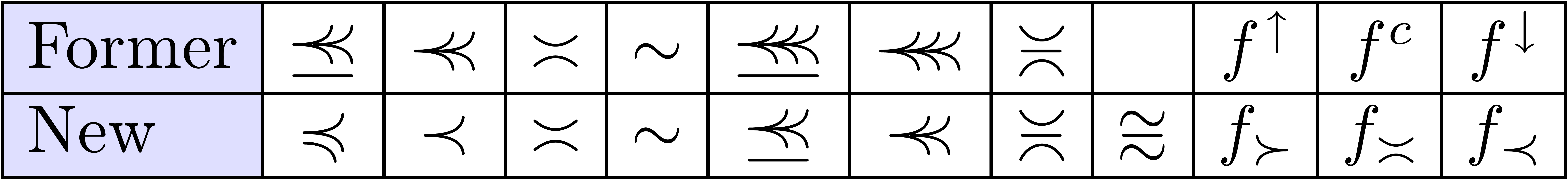
There are also a few changes in terminology:
| Former | New |
| normal basis | transbasis |
| purely exponential transseries | exponential transseries |
| potential dominant — | starting — |
| privileged refinement |  unravelling unravelling |
In this chapter, we will introduce some order-theoretical concepts, which prepare the study of generalized power series in the next chapter. Orderings occur in at least two important ways in this study.
First, the terms of a series are naturally ordered according to their
asymptotic magnitudes. For instance, the support of  , considered as an ordered set, is isomorphic
to
, considered as an ordered set, is isomorphic
to  . More interesting
examples are
. More interesting
examples are

and

whose supports are isomorphic to  and
and  respectively. Here denotes the set
 with the total anti-lexicographical ordering

and denotes the set with
the partial product ordering

In general, when the support is totally ordered, it is natural to require the support to be well-ordered. If we want to be able to multiply series, this condition is also necessary, as shown by the example

For convenience, we recall some classical results about well-ordered sets and ordinal numbers in section 1.2. In what follows, our treatment will be based on well-quasi-orderings, which are the analogue of well-orderings in the context of partial quasi-orderings. In sections 1.3 and 1.4, we will prove some classical results about well-quasi-orderings.
A second important occurrence of orderings is when we consider an
algebra of generalized power series as an ordered structure. For
instance  is naturally ordered by declaring a
non-zero series
is naturally ordered by declaring a
non-zero series  with
with  to
be positive if and only if
to
be positive if and only if  .
This gives the structure of a so called totally
ordered -algebra.
.
This gives the structure of a so called totally
ordered -algebra.
In section 1.5, we recall the definitions of several types
of ordered algebraic structures. In section 1.6, we will
then show how a certain number of typical asymptotic relations, like
 , ,
, ,  and
and  , can be introduced in a purely algebraic way. In
section 1.8, we define groups and fields with generalized
exponentiations, and the asymptotic relations
, can be introduced in a purely algebraic way. In
section 1.8, we define groups and fields with generalized
exponentiations, and the asymptotic relations  ,
, 
 and
and  . Roughly speaking, for
infinitely large and
. Roughly speaking, for
infinitely large and  , we have
  ,
if
,
if  for all
  .
For instance,
.
For instance,  , but
, but  , for
, for  .
.
Let  be a set. In all what follows, a
quasi-ordering on is
reflexive and transitive relation
be a set. In all what follows, a
quasi-ordering on is
reflexive and transitive relation  on ; in other words,
for all
on ; in other words,
for all  we have
 ;
;
 .
.
An ordering is a quasi-ordering which is also antisymmetric:
 .
.
We sometimes write  instead of
in order to avoid confusion. A mapping
instead of
in order to avoid confusion. A mapping  between
two quasi-ordered sets is said to be increasing (or
a morphism of quasi-ordered sets), if
between
two quasi-ordered sets is said to be increasing (or
a morphism of quasi-ordered sets), if  ,
for all
,
for all  .
.
Given a quasi-ordering , we
say that are comparable if
 or
or  .
If every two elements in are comparable, then
the quasi-ordering is said to be total.
Two elements
.
If every two elements in are comparable, then
the quasi-ordering is said to be total.
Two elements  are said to be
equivalent, and we write
are said to be
equivalent, and we write  , if and . If and
  , then we write
  (see
also exercise 1.1(a) below). The quasi-ordering on induces a natural ordering on the quotient set
(see
also exercise 1.1(a) below). The quasi-ordering on induces a natural ordering on the quotient set  by
by  and the corresponding
projection
and the corresponding
projection  is increasing. In other words, we do
not really gain in generality by considering quasi-orderings instead of
orderings, but it is sometimes more convenient to deal with
quasi-orderings.
is increasing. In other words, we do
not really gain in generality by considering quasi-orderings instead of
orderings, but it is sometimes more convenient to deal with
quasi-orderings.
Some simple examples of totally ordered sets are  and . Any set can be trivially quasi-ordered both by the finest
ordering, for which
and . Any set can be trivially quasi-ordered both by the finest
ordering, for which  ,
and by the roughest quasi-ordering, for which all satisfy . In
general, a quasi-ordering on
is said to be finer than a second quasi-ordering
,
and by the roughest quasi-ordering, for which all satisfy . In
general, a quasi-ordering on
is said to be finer than a second quasi-ordering
 on if
on if  for all . Given quasi-ordered
sets and
for all . Given quasi-ordered
sets and  ,
we can construct other quasi-ordered sets as follows:
,
we can construct other quasi-ordered sets as follows:
The disjoint union  is naturally quasi-ordered, by taking the quasi-orderings on and on each summand, and
by taking and
mutually incomparable. In other words,
is naturally quasi-ordered, by taking the quasi-orderings on and on each summand, and
by taking and
mutually incomparable. In other words,

Alternatively, we can quasi-order
, by postulating any
element in to be strictly smaller than any
element in . This
quasi-ordered set is called the ordered union of
and , and we denote it by
 . In other words,

The Cartesian product  is naturally quasi-ordered by

Alternatively, we can quasi-order
anti-lexicographically by

We write  for the corresponding quasi-ordered
set.
for the corresponding quasi-ordered
set.
Let  be the
set of words over .
Such words are denoted by sequences
be the
set of words over .
Such words are denoted by sequences  (with
(with
 ) or
) or  if confusion may arise. The empty word is denoted by
  and we define
  . The
embeddability quasi-ordering on is defined by
. The
embeddability quasi-ordering on is defined by  ,
if and only if there exists a strictly increasing mapping
,
if and only if there exists a strictly increasing mapping  , such that
  for all . For instance,

An equivalence relation on
is said to be compatible with the quasi-ordering
if

for all  . In that case,
 is naturally quasi-ordered by

and the canonical projection  is increasing.
If and are ordered sets,
then it can be verified that the quasi-orderings defined in 1–6
above are actually orderings.
Let be an increasing mapping between
quasi-ordered sets  and
and  . Consider the quasi-ordering
on defined by
. Consider the quasi-ordering
on defined by

Then is finer than and
the mapping  admits a natural factorization
 |
(1.1) |
Here  is the identity on
composed with the natural projection from
is the identity on
composed with the natural projection from  on
on
 ,
,  is
the natural inclusion of
is
the natural inclusion of  into
and
into
and  is an isomorphism.
A strict ordering on
is a transitive and antireflexive relation  on (i.e.
  for no elements
  ).
Given a quasi-ordering show that the
relation defined by
).
Given a quasi-ordering show that the
relation defined by  is a strict ordering. Show also how to associate an ordering to a
strict ordering.
is a strict ordering. Show also how to associate an ordering to a
strict ordering.
Let  be a
quasi-ordering on .
Show that the relation
be a
quasi-ordering on .
Show that the relation  defined by
  is also a quasi-ordering on ; we call it the opposite
quasi-ordering of .
is also a quasi-ordering on ; we call it the opposite
quasi-ordering of .
Let be a quasi-ordering on . Show that  defines an ordering on .
Show that
defines an ordering on .
Show that  is the roughest ordering which
is finer than .
is the roughest ordering which
is finer than .
Exercise 1.2. Two
quasi-ordered sets  and
and  are said to be isomorphic, and we write
  , if there is an increasing bijection between
and ,
whose inverse is also increasing. Prove the following:
, if there is an increasing bijection between
and ,
whose inverse is also increasing. Prove the following:
 and
and  are
commutative modulo
are
commutative modulo  (i.e.
(i.e.
 ), but not
  and
and  .
.
 and
and  are
associative modulo .
are
associative modulo .
is distributive w.r.t. modulo .
is right (but not left) distributive
w.r.t. modulo (in other words  ).
).
Exercise 1.3. Let be a quasi-ordered set. We define
an equivalence relation on ,
by taking two words to be equivalent if they are obtained one from
another by a permutation of letters. We call  the set of commutative words over . Show that:
We define a quasi-ordering on by  .
.
For all  , we have
  if and only if there exists an injection
  with for all .
The equivalence relation is compatible
with , so that we may
order  by the quotient quasi-ordering
induced by .
by the quotient quasi-ordering
induced by .
The quasi-ordering is finer than and we have a natural increasing surjection  .
.
For all ordered sets  ,
prove that
,
prove that  .
.
For all ordered sets prove that there
exists an increasing bijection  ,
whose inverse is not increasing, in general.
,
whose inverse is not increasing, in general.

Prove that  defines an ordering on
 . Also prove the following
properties:
. Also prove the following
properties:
If  , then
  .
.
If  , then
  .
.
 .
.
 .
.
Exercise 1.5. Show that the category of quasi-ordered sets admits direct sums and products, pull-backs, push-outs, direct and inverse limits and free objects (i.e. the forgetful functor to the category of sets admits a right adjoint).
Let be a quasi-ordered set. The quasi-ordering
on is said to be well-founded, if there is no infinite strictly decreasing sequence in . A total well-founded ordering is
called a well-ordering. A total ordering is a
well-ordering if and only if each of its non-empty subsets has a least
element. The following classical theorems are implied by the axiom of
choice [Bou70, Mal79]:
Theorem 1.1. Every set can be well-ordered.
Theorem 1.2. be a non-empty
ordered set, such that each non-empty totally ordered subset of has an upper bound. Then
admits a maximal element.
An ordinal number or ordinal is a set  , such that the relation
  forms a strict well-ordering on . In particular, the natural numbers can “be
defined to be” ordinal numbers:
forms a strict well-ordering on . In particular, the natural numbers can “be
defined to be” ordinal numbers:  .
The set
.
The set  of natural numbers is also an
ordinal. More generally, if is an ordinal, then
so is
of natural numbers is also an
ordinal. More generally, if is an ordinal, then
so is  . For all ordinals
, its elements are also
ordinals.
. For all ordinals
, its elements are also
ordinals.
It is classical [Mal79] that the class of all ordinal
numbers has all the properties of an ordinal number: if  and
and  are ordinal numbers, then
  and each non-empty set of ordinals admits a least element for . The following classification
theorem is also classical [Mal79]:
and each non-empty set of ordinals admits a least element for . The following classification
theorem is also classical [Mal79]:
Theorem 1.3. Each well-ordered set is isomorphic to
a unique ordinal.
The usual induction process for natural numbers admits an analogue for
ordinal numbers. For this purpose, we distinguish between successor
ordinals and limit ordinals: an ordinal is
called a successor ordinal if  for some ordinal
  (and we write
  ) and a limit ordinal if
not (in which case
) and a limit ordinal if
not (in which case  ). For
example, the inductive definitions for addition, multiplication and
exponentiation can now be extended to ordinal numbers as follows:
). For
example, the inductive definitions for addition, multiplication and
exponentiation can now be extended to ordinal numbers as follows:
Similarly, one has the transfinite induction
principle: assume that a property for ordinals
satisfies  for all and
 for all limit ordinals . Then
  holds for all
ordinals .
holds for all
ordinals .
The following theorem classifies all countable ordinals smaller than
, and is due to Cantor [Can99]:
Theorem 1.4. Let
 be a countable ordinal. Then there exists a
unique sequence of natural numbers
be a countable ordinal. Then there exists a
unique sequence of natural numbers  (with
(with  if
if  ), such
that
), such
that


Exercise 1.6. Prove the transfinite induction principle.
Exercise 1.7. For any two ordinals  , show that
 ;
;
 .
.
In particular,  and
and  are associative and is right
distributive w.r.t. ,
by exercise 1.2.
are associative and is right
distributive w.r.t. ,
by exercise 1.2.
Exercise 1.8. For all ordinals and  , prove
that
, prove
that
 ;
;
 .
.
Do we also have  ?
?
Let be a quasi-ordered set. A chain in is a subset of
which is totally ordered for the induced quasi-ordering. An
anti-chain is a subset of of
pairwise incomparable elements. A well-quasi-ordering is a well-founded quasi-ordering without infinite anti-chains.
A final segment is a subset
of , such that  , for all .
Given an arbitrary subset
, for all .
Given an arbitrary subset  of , we denote by

the final segment generated by .
Dually, an initial segment is a subset of , such that
 , for all . We denote by

the initial segment generated by .
Proposition 1.5. Let
be a quasi-ordered set. Then the following are equivalent:
is well-quasi-ordered.
Any final segment of is finitely
generated.
The ascending chain condition w.r.t. inclusion holds
for final segments of .
Each sequence  admits an increasing
subsequence.
admits an increasing
subsequence.
Any extension of the quasi-ordering on to
a total quasi-ordering on yields a
well-founded quasi-ordering.
Proof. Assume (a) and let be a
final segment of and  the
subset of minimal elements of .
Then
the
subset of minimal elements of .
Then  is an anti-chain, whence finite. We claim
that generates .
Indeed, in the contrary case, let
is an anti-chain, whence finite. We claim
that generates .
Indeed, in the contrary case, let  .
Since
.
Since  is not minimal in , there exists an
  with
with  . Repeating this argument, we
obtain an infinite decreasing sequence
. Repeating this argument, we
obtain an infinite decreasing sequence  .
This proves (b). Conversely, if
.
This proves (b). Conversely, if  is an
infinite anti-chain or an infinite strictly decreasing sequence, then
the final segment generated by
is an
infinite anti-chain or an infinite strictly decreasing sequence, then
the final segment generated by  is not finitely
generated. This proves (a)
is not finitely
generated. This proves (a) (b).
(b).
Now let  be an ascending chain of final segments.
If the final segment
be an ascending chain of final segments.
If the final segment  is finitely generated, say
by , then we must have
is finitely generated, say
by , then we must have  , for some
  . This shows that (b)
 (c). Conversely, let
be the set of minimal elements of a final segment . If
(c). Conversely, let
be the set of minimal elements of a final segment . If  ,…
are pairwise distinct elements of ,
then
,…
are pairwise distinct elements of ,
then  forms an infinite strictly ascending chain
of final segments.
forms an infinite strictly ascending chain
of final segments.
Now consider a sequence of elements in , and assume that
is a well-quasi-ordering. We extract an increasing sequence  from it by the following procedure: Let
  be the final segment generated by the
  ,
with
,
with  and
and  (
( by convention) and assume by induction that the sequence
contains infinitely many terms in . Since is finitely
generated by (b), we can select a generator
by convention) and assume by induction that the sequence
contains infinitely many terms in . Since is finitely
generated by (b), we can select a generator  , with
  and such that
the sequence contains infinitely many terms in
and such that
the sequence contains infinitely many terms in
 . This implies (d). On
the other hand, it is clear that it is not possible to extract an
increasing sequence from an infinite strictly decreasing sequence or
from a sequence of pairwise incomparable elements.
. This implies (d). On
the other hand, it is clear that it is not possible to extract an
increasing sequence from an infinite strictly decreasing sequence or
from a sequence of pairwise incomparable elements.
Let us finally prove (a)(e).
An ordering containing an infinite anti-chain or an infinite strictly
decreasing sequence can always be extended to a total quasi-ordering
which contains a copy of  , by
a straightforward application of Zorn's lemma. Inversely, any extension
of a well-quasi-ordering is a well-quasi-ordering.
, by
a straightforward application of Zorn's lemma. Inversely, any extension
of a well-quasi-ordering is a well-quasi-ordering.
The most elementary examples of well-quasi-orderings are well-orderings and quasi-orderings on finite sets. Other well-quasi-orderings can be constructed as follows.
Proposition 1.6. Assume that and are well-quasi-ordered sets.
Then
Any subset of with the induced ordering is
well-quasi-ordered.
Let be a morphism of ordered sets. Then
is well-quasi-ordered.
Any ordering on which extends is a well-quasi-ordering.
 is well-quasi-ordered, for any compatible
equivalence relation on .
is well-quasi-ordered, for any compatible
equivalence relation on .
and are
well-quasi-ordered.
and are
well-quasi-ordered.
Proof. Properties (a), (b), (e) and
(f) follow from proposition 1.5(d). The
properties (c) and (d) are special cases of
(b).
Corollary 1.7.  ,
the set
,
the set  with the partial, componentwise ordering
is a well-quasi-ordering.
with the partial, componentwise ordering
is a well-quasi-ordering.
Theorem 1.8. is be a well-quasi-ordered
set. Then is a well-quasi-ordered set.
Proof. Our proof is due to Nash-Williams [NW63]. If
denotes any ordering, then we say that  is a bad sequence, if there do not
exist
is a bad sequence, if there do not
exist  with
with  .
A quasi-ordering is a well-quasi-ordering, if and only if there are no
bad sequences.
.
A quasi-ordering is a well-quasi-ordering, if and only if there are no
bad sequences.
Now assume for contradiction that  is a bad
sequence for
is a bad
sequence for  . Without loss
of generality, we may assume that each
. Without loss
of generality, we may assume that each  was
chosen such that the length (as a word) of were
minimal, under the condition that
was
chosen such that the length (as a word) of were
minimal, under the condition that

We say that  is a minimal bad sequence.
Now for all  , we must have
 , so we can factor
  , where
  is
the first letter of . By
proposition 1.5(d), we can extract an increasing
sequence from .
Now consider the sequence
is
the first letter of . By
proposition 1.5(d), we can extract an increasing
sequence from .
Now consider the sequence

By the minimality of  , this
sequence is good. Hence, there exist
, this
sequence is good. Hence, there exist  with
with  . But then,

which contradicts the badness of .
Exercise 1.9. Show that
is a well-quasi-ordering if and only if the ordering on  is a well-quasi-ordering.
Exercise 1.10. Prove the principle of
Noetherian induction: let  be a property for well-quasi-ordered sets, such that
 holds, whenever holds
for all proper initial segments of .
Then holds for all well-quasi-ordered
sets.
holds, whenever holds
for all proper initial segments of .
Then holds for all well-quasi-ordered
sets.
Exercise 1.11. Let
and be well-quasi-ordered sets. With  as in exercise 1.4, when is also well-quasi-ordered?
Exercise 1.12. Let
be a well-quasi-ordered set. The set  of
initial segments of is naturally ordered by
inclusion. Show that is not necessarily
well-quasi-ordered. We define to be a strongly
well-quasi-ordered set if is also
well-quasi-ordered. Which properties from proposition 1.6
generalize to strongly well-quasi-ordered sets?
of
initial segments of is naturally ordered by
inclusion. Show that is not necessarily
well-quasi-ordered. We define to be a strongly
well-quasi-ordered set if is also
well-quasi-ordered. Which properties from proposition 1.6
generalize to strongly well-quasi-ordered sets?
Exercise 1.13. A limit
well-quasi-ordered set is a well-quasi-ordered set , such that there are no final segments of
cardinality 1. Given two well-quasi-ordered sets
and , we define and to be equivalent if there
exists an increasing injection from into and vice versa. Prove that a limit
well-quasi-ordered set is equivalent to a unique limit ordinal.
An unoriented tree is a finite set  of nodes with a partial ordering
  , such that
admits a minimal element
, such that
admits a minimal element  ,
called the root of , and
such that each other node admits a predecessor. Given
,
called the root of , and
such that each other node admits a predecessor. Given  , we recall that
  is a
predecessor of
is a
predecessor of  (and a successor of ) if
  and
and
 for any
  with
with  . A node without successors is
called a leaf. Any
node
. A node without successors is
called a leaf. Any
node  naturally induces a subtree
 with root .
Since is finite, an easy induction shows that
any two nodes
with root .
Since is finite, an easy induction shows that
any two nodes  of admit
an infimum
of admit
an infimum  w.r.t. , for
which
w.r.t. , for
which  ,
,  and
and  for all
  with and
  .
.
An oriented tree (or simply tree) is an
unoriented tree , together
with a total ordering  which extends and which satisfies the condition

It is not hard to see that such a total ordering
is uniquely determined by its restrictions to the sets of -successors for each node .
Two unoriented or oriented trees and  will be understood to be equal if there exists a bijection
 which preserves
resp. and
which preserves
resp. and  . In particular, under this identification, the sets
of unoriented and oriented trees are countable.
. In particular, under this identification, the sets
of unoriented and oriented trees are countable.
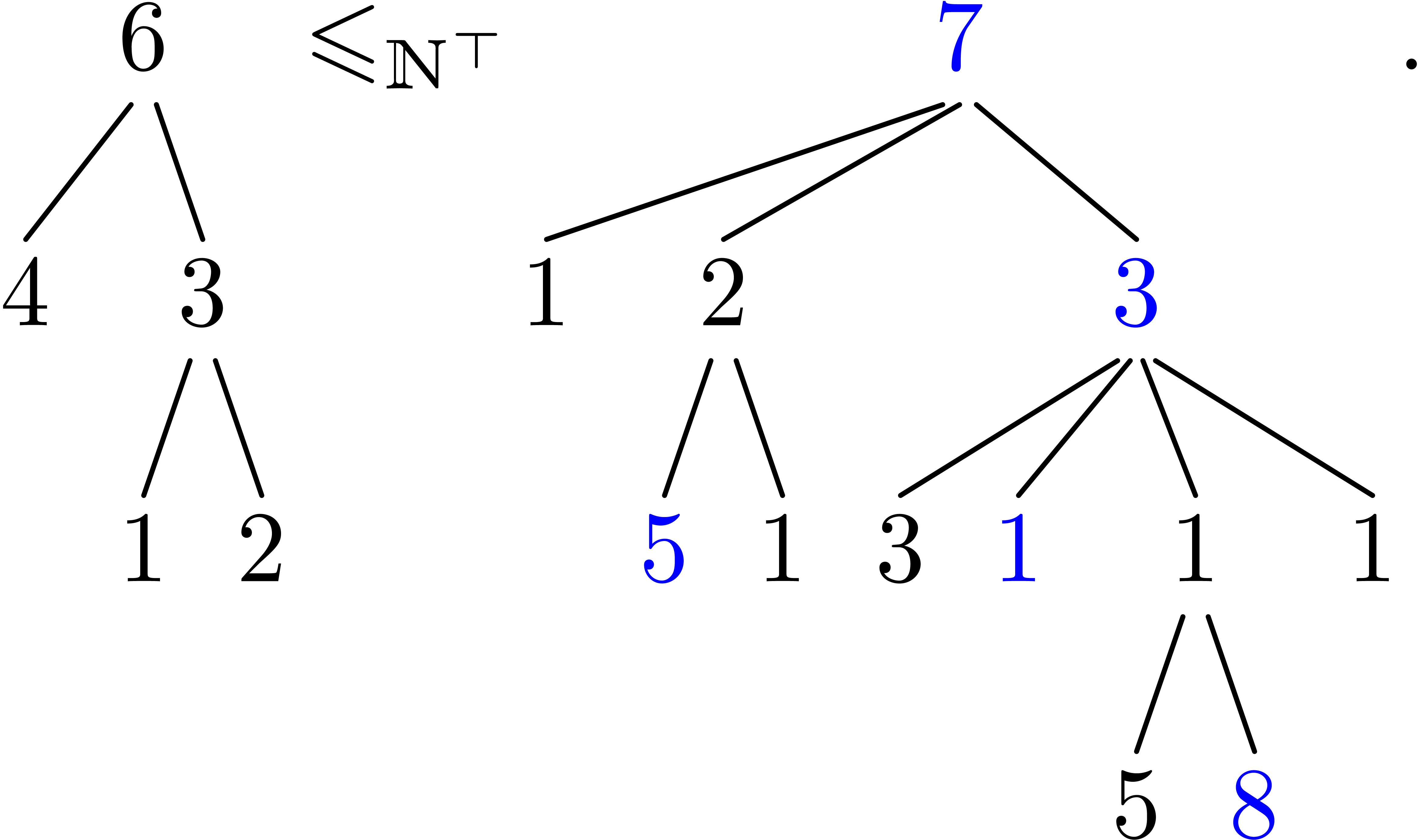
Given a set , an -labeled tree is a
tree together with a labeling  . We denote by
  the set of such trees. An -labeled
tree may be represented graphically by
the set of such trees. An -labeled
tree may be represented graphically by
 |
(1.2) |
where  and
and  are the
subtrees associated to the successors
are the
subtrees associated to the successors  of . We call
  the children of the root and
  its arity. Notice that we may have
  .
.
Example 1.9. We may see usual trees as  -labeled trees, where is the
set with one symbolic element
-labeled trees, where is the
set with one symbolic element  .
The difference between unoriented and oriented trees is that the
ordering on the branches is important. For instance, the two trees below
are different as oriented trees, but the same as unoriented trees:
.
The difference between unoriented and oriented trees is that the
ordering on the branches is important. For instance, the two trees below
are different as oriented trees, but the same as unoriented trees:

If is a quasi-ordered set, then the
embeddability quasi-ordering on is defined by  ,
if and only if there exists a strictly increasing mapping
,
if and only if there exists a strictly increasing mapping  for , such that
 , and
, and  , for all
  .
An example of a tree which embeds into another tree is given by
.
An example of a tree which embeds into another tree is given by
The following theorem is known as Kruskal's theorem:
Theorem 1.10. If
is a well-quasi-ordered set, then so is .
Proof. Assume that there exists a bad sequence  . We may assume that we have chosen each

of minimal cardinality (assuming that  have
already been fixed), i.e. is a
“minimal bad sequence”. We claim that the induced
quasi-ordering on
have
already been fixed), i.e. is a
“minimal bad sequence”. We claim that the induced
quasi-ordering on  is a well-quasi-ordering.
Indeed, suppose the contrary, and let
is a well-quasi-ordering.
Indeed, suppose the contrary, and let

be a bad sequence. Let  be such that
  is minimal. Then the sequence

is also bad, which contradicts the minimality of . Hence,  is
well-quasi-ordered, and so is
is
well-quasi-ordered, and so is  ,
by Higman's theorem and proposition 1.6(f). But each
tree
,
by Higman's theorem and proposition 1.6(f). But each
tree  can be interpreted as an element of . Hence,
  is
a well-quasi-ordered subset of ,
which contradicts our assumption that is a bad
sequence.
is
a well-quasi-ordered subset of ,
which contradicts our assumption that is a bad
sequence.
Remark 1.11. In the case when we restrict ourselves to trees of bounded arity, the above theorem was already due to Higman. The general theorem was first conjectured by Vázsonyi. The proof we have given here is due to Nash-Williams.
Exercise 1.14. Let  be a quasi-ordered set and let
  be an ordered
set of operations on . That
is, the elements of are mappings
be an ordered
set of operations on . That
is, the elements of are mappings  . We say that such an operation is extensive, if for all
  and
and  , we
have
, we
have

We say that the orderings of and
are compatible, if for all  , and
, and
 , we have

whenever there exists an increasing mapping  with
with  for all .
Assume that these conditions are satisfied and let be a subset of .
The smallest subset of which contains and which is stable under
is said to be the subset of generated
by w.r.t. , and will be denoted by  . If is a
well-quasi-ordered subset of and the ordering
on is well-quasi-ordered, then prove that is well-quasi-ordered.
. If is a
well-quasi-ordered subset of and the ordering
on is well-quasi-ordered, then prove that is well-quasi-ordered.
In what follows, all monoids, groups and rings will be commutative and all rings unitary. The following ordered structures will be encountered frequently throughout this book. Recall that we systematically understand all orderings to be partial (contrary to what is customary for certain structures).
An ordered monoid is a monoid  with an ordering such that

for all  . If is rather an additive monoid (in which case is assumed to be abelian), then OM
becomes
. If is rather an additive monoid (in which case is assumed to be abelian), then OM
becomes
 .
.
An ordered ring is a ring  with an ordering with the following
properties:
with an ordering with the following
properties:
 ;
;
;
 ,
,
for all  .
.
An ordered field is a field  with an ordering which makes an ordered ring and such that
  for all
  . Notice that
this latter condition is automatically satisfied if
is total.
. Notice that
this latter condition is automatically satisfied if
is total.
An ordered -module over an ordered ring is an -module  with an ordering which satisfies
;
 ,
,
for all  and
and  .
Any abelian group is trivially an ordered
.
Any abelian group is trivially an ordered  -module.
An ordered -algebra is a morphism  of ordered rings,
i.e. an increasing ring morphism of an ordered ring
into an ordered ring . As usual, we denote
of ordered rings,
i.e. an increasing ring morphism of an ordered ring
into an ordered ring . As usual, we denote  , for and
  . Notice that is in
particular an ordered -module.
Any ordered ring is trivially an ordered
-algebra.
. Notice that is in
particular an ordered -module.
Any ordered ring is trivially an ordered
-algebra.
Let be an ordered abelian group, ring, -module or -algebra. We denote

We observe that the ordering is characterized by
 . If
is totally ordered, then we define the absolute value
of
. If
is totally ordered, then we define the absolute value
of  by
by  if
if  and
and  , if
, if  .
.
Example 1.12.  and
and  are the most common examples of totally ordered fields.
  and
and  are respectively a totally ordered monoid
and a totally ordered group. The complex numbers form an ordered abelian
group when setting
are respectively a totally ordered monoid
and a totally ordered group. The complex numbers form an ordered abelian
group when setting  . However,
this ordering is partial and not compatible with the multiplication.
Notice that
. However,
this ordering is partial and not compatible with the multiplication.
Notice that  and
and  are
incomparable for
are
incomparable for  and
and  .
.
Example 1.13. The ring of germs at  of infinitely differentiable real valued functions on intervals
  with
with  can be ordered by
  , if there exists an
  , such that
  for all
 . A totally ordered subfield
of this ring is called a Hardy field.
. A totally ordered subfield
of this ring is called a Hardy field.
Example 1.14. The above definitions naturally generalize to the
case of quasi-orderings instead of orderings. If  is a quasi-ordered abelian group, then
  is an
ordered abelian group, and similarly for quasi-ordered rings,
is an
ordered abelian group, and similarly for quasi-ordered rings,  -modules, etc.
Example 1.15. Let and  be two quasi-ordered abelian groups, rings, -modules or -algebras.
Their direct sum
be two quasi-ordered abelian groups, rings, -modules or -algebras.
Their direct sum  is
naturally quasi-ordered by the product quasi-ordering
is
naturally quasi-ordered by the product quasi-ordering

Similarly, the anti-lexicographical direct sum
 of and
is
of and
is  with the anti-lexicographical quasi-ordering

If and are ordered, then
so are  and
and  .
.
Example 1.16. Let and
be two quasi-ordered abelian groups, rings, -modules or -algebras.
Their tensor product  is
naturally quasi-ordered, by declaring an element of
to be positive if it is a sum of elements of the form
is
naturally quasi-ordered, by declaring an element of
to be positive if it is a sum of elements of the form  with
with  and
and  .
Similarly, we define the anti-lexicographical tensor product
.
Similarly, we define the anti-lexicographical tensor product  : its set
of positive elements is additively generated by elements in of the form
: its set
of positive elements is additively generated by elements in of the form  ,
with
,
with  and
and  .
If and are ordered, then
the same does not necessarily hold for
.
If and are ordered, then
the same does not necessarily hold for
Exercise 1.15. Let
be a totally ordered integral domain and let  be its quotient field.
Show that  , for all
 .
.
If  is a total ordering, then show that
there exists a unique total ordering on , which extends
is a total ordering, then show that
there exists a unique total ordering on , which extends  ,
and for which is an ordered field.
,
and for which is an ordered field.
Show that  , for all
. In particular, if
contains no nilpotent elements, then is an integral domain.
, for all
. In particular, if
contains no nilpotent elements, then is an integral domain.
Show that may contain nilpotent elements.
Show that may contain zero divisors which
are not nilpotent.
Show that positive non-nilpotent elements are larger than any
nilpotent element in .
Exercise 1.17. Let  and
and  be quasi-ordered rings. Prove the
following properties:
be quasi-ordered rings. Prove the
following properties:
 and
and  ;
;
 and
and  ;
;
 and
and  ;
;
 , but not always
  .
.
Show that the categories of ordered abelian groups, rings, -modules and -algebras (its morphisms are increasing
morphisms of abelian groups, rings, etc.) admit direct sums and
products, pull-backs, push-outs, direct and inverse limits and
free objects (i.e. the forgetful functor to the
category of sets admits a right adjoint).
Show that the same thing holds for the categories of ordered
torsion free groups, rings without nilpotent elements, torsion
free -modules and
ordered -algebras without nilpotent elements, and such that the
mapping  is injective.
What can be said about the operations  and
and
 introduced above?
Exercise 1.19. Let
be an ordered abelian group, ring, -module
or -algebra. We wish to
investigate under which circumstances the ordering
can be extended into a total ordering.
If is an ordered abelian monoid, prove
that can be extended into a total ordering
if and only if is torsion free
(i.e.  ,
for all
,
for all  and ).
Hint: use Zorn's lemma.
and ).
Hint: use Zorn's lemma.
If is an ordered ring without nilpotent
elements, prove that can be extended into
a total ordering if and only if is an
integral domain, such that

for all  , such that
. Hint: first reduce
the problem to the case when all squares in
are positive. Next reduce the problem to the case when
, such that
. Hint: first reduce
the problem to the case when all squares in
are positive. Next reduce the problem to the case when  , for all
  .
.
Generalize b to the case when is an
ordered ring, which may contain nilpotent elements.
Give conditions in the cases when is an
ordered -module or an
ordered -algebra
without nilpotent elements.
Exercise 1.20. Let
be an ordered group, ring, -module
or -algebra. For each
morphism  of into a
totally ordered structure
of into a
totally ordered structure  of the same kind as
, we define a relation
of the same kind as
, we define a relation  on by
on by  . Let be the set of
all such relations on .
. Let be the set of
all such relations on .
Prove that  is a quasi-ordering.
Show that  is an ordering, if and only if
can be extended into a total ordering on
.
is an ordering, if and only if
can be extended into a total ordering on
.
Let  the equivalence relation associated to
and let
the equivalence relation associated to
and let  .
Show that the ordered set
.
Show that the ordered set  can be given the
same kind of ordered algebraic structure as , in such a way that the natural projection
can be given the
same kind of ordered algebraic structure as , in such a way that the natural projection
 is a morphism. We call
the closure of .
is a morphism. We call
the closure of .
is said to be perfect
if is a bijection. Prove that the closure
of is perfect.
Show that an ordered abelian group is
perfect if and only if  ,
for all and .
,
for all and .
Show that an ordered ring without nilpotent elements is perfect,
if and only if  , for
all and
, for
all and  ,
for all .
,
for all .
Under which conditions is an ordered -module
perfect? And an ordered -algebra
without nilpotent elements?
Let and be two germs of
real valued functions at infinity. Then we have the following classical
definitions of the domination and neglection relations
resp. :

Considered as relations on the -algebra
of germs of real valued functions at infinity,
and satisfy a certain number of easy to prove
algebraic properties. In this section, we will take these properties as
the axioms of abstract domination and neglection relations on more
general modules and algebras.
Let be a ring and an
-module. In all what follows,
we denote by  the set of
non-zero-divisors in . A
dominance relation is a quasi-ordering
on ,
such that for all ,
the set of
non-zero-divisors in . A
dominance relation is a quasi-ordering
on ,
such that for all ,  and
and  , we have
 ;
;
 and
and
 .
.
Notice that D1 and D2 imply that  is a submodule of for each
  . If
. If  ,
then we say that is dominated
by
,
then we say that is dominated
by  , and we also write
  . If and
  , then we say that
and are asymptotic, and we
also write
, then we say that
and are asymptotic, and we
also write  . We say that is total, if
or for all
. We say that is total, if
or for all  .
.
A neglection relation is a strict
ordering on
(i.e. an anti-reflexive, transitive relation), such that
for all and and , we have
 ;
;
 and
and
 .
.
 .
.
Notice that  is a submodule of
if
is a submodule of
if  . However, this is not
always the case, since
. However, this is not
always the case, since  . If
. If
 , then we say that can be neglected w.r.t. , and we also write
  . If
. If  ,
then we also say that and
are equivalent, and we write
,
then we also say that and
are equivalent, and we write  . Indeed, is an equivalence relation:

Similarly,

whence

We say that is compatible with a dominance relation , if  and
and  , for all .
In that case, we call an asymptotic -module. We say
that and are
associated, if is the strict ordering associated to , i.e.
, for all .
In that case, we call an asymptotic -module. We say
that and are
associated, if is the strict ordering associated to , i.e.  for
all .
for
all .
Let be a dominance relation such that the
strict ordering associated to satisfies also
satisfies
Let and be a
dominance and a neglection relation. If
and are associated, then they are
compatible.
Proof. Assume that  satisfies the
condition in (a), and let
satisfies the
condition in (a), and let  be such that
 and
and  .
If
.
If  , then
  implies
  and
and  :
contradiction. Hence, we have
:
contradiction. Hence, we have  and
and  .
.
As to (b), assume that and  are associated. Then we clearly have
  . Furthermore,
  .
Similarly,
.
Similarly,  . Hence,
  .
.
Proposition 1.18. Let
be a totally ordered field and  an ordered -vector space. Then is an asymptotic -vector
space for the relations and
defined by
an ordered -vector space. Then is an asymptotic -vector
space for the relations and
defined by

Moreover, if is totally ordered, then is associated to .
Proof. Let us first show that is a
quasi-ordering. We clearly have  for all
  , since
  for
all
for
all  . If
. If  and , then there exists a
 with
with  and a
and a  with
with  . Let us
next prove D1. Assume that
. Let us
next prove D1. Assume that  and
and  and let . Then
there exist
and let . Then
there exist  with
with  and
and
 , whence
  . As to D2, let ,
  and
and  . Then for all ,
we have
. Then for all ,
we have  and
and  .
.
In order to prove the remaining relations, we first notice that

Indeed, if  , then there
exists a with
, then there
exists a with  for all
 . In particular,
  , whence either
  (if
(if
 ) or
) or  (if
(if  ). Furthermore, for all
, we have
). Furthermore, for all
, we have  , whence
  .
Let us show that is a strict ordering. We cannot
have
.
Let us show that is a strict ordering. We cannot
have  , since
  . If
. If  ,
then we have
,
then we have  for all .
Let us now prove N1. If ,
and ,
then  and
and  ,
whence
,
whence  . As to N2, let
, and
. If , then
. As to N2, let
, and
. If , then  ,
whence
,
whence  . If
. If  , then
  and
and  , whence .
Let us finally prove N3. Assume that , and . Then
, whence .
Let us finally prove N3. Assume that , and . Then  implies
  . From it thus follows
that
. From it thus follows
that  .
.
Assuming that is totally ordered, the relation
is associated to ,
since  . In general, we
clearly have . Furthermore,
if
. In general, we
clearly have . Furthermore,
if  , then both
  and
and  , whence
 . Similarly,
  , so that
  .
.
If is a totally ordered ring, then cannot have zero-divisors, so its ring of quotients  is a totally ordered field. Moreover, for any
ordered, torsion-free -module,
the natural map
is a totally ordered field. Moreover, for any
ordered, torsion-free -module,
the natural map  is an embedding. This allows us
to generalize proposition 1.18 to the case of totally
ordered rings.
is an embedding. This allows us
to generalize proposition 1.18 to the case of totally
ordered rings.
Corollary 1.19. Let
be a totally ordered ring and  an ordered,
torsion-free -module. Then
is an asymptotic -module
for the restrictions to of the relations and on
an ordered,
torsion-free -module. Then
is an asymptotic -module
for the restrictions to of the relations and on  . Moreover, if is totally
ordered, then is associated to .
. Moreover, if is totally
ordered, then is associated to .
Assume now that is an -algebra. A dominance relation on
is defined to be a quasi-ordering ,
which satisfies D1, D2 and for all  :
:
 .
.
A neglection relation on is a strict ordering
, which satisfies N1,
N2, N3, and for all  and
and  :
:
 .
.
An element is said to be
infinitesimal, if  .
We say that is bounded, if
.
We say that is bounded, if
 (and unbounded if not).
Elements with
(and unbounded if not).
Elements with  are called archimedean. If all non-zero elements of are
archimedean, then is said to be
archimedean itself. In particular, a
totally ordered ring said to be archimedean, if it is archimedean as an
ordered -algebra. If and are compatible, then we
call an asymptotic -algebra.
are called archimedean. If all non-zero elements of are
archimedean, then is said to be
archimedean itself. In particular, a
totally ordered ring said to be archimedean, if it is archimedean as an
ordered -algebra. If and are compatible, then we
call an asymptotic -algebra.
Proposition 1.20. Let
be a totally ordered ring and a non-trivial
totally ordered -algebra.
Define the relations and
on as in corollary 1.19. Then is an asymptotic -algebra
and is associated to .
Proof. Let  be such that
  , and let
  .
Then there exists a
.
Then there exists a  with . If
  ,
then we infer that
,
then we infer that  , whence
 . If
. If  , then we obtain
  ,
whence again , by D2.
This proves D3. As to N4, let be
such that . Then for all
, we have
,
whence again , by D2.
This proves D3. As to N4, let be
such that . Then for all
, we have  , whence
  .
.
Example 1.21. Let be a totally ordered
-algebra. We may totally
order the polynomial extension  of by an infinitesimal element
  by
setting
by
setting  , if and only if
there exists an index
, if and only if
there exists an index  with
with  . This algebra is non-archimedean, since
  . Similarly, one may construct an
extension
. Similarly, one may construct an
extension  with an infinitely large element
  , in which
  .
.
Given a totally ordered vector space  over
a totally ordered field ,
show that
over
a totally ordered field ,
show that

Given a totally ordered module over a
totally ordered ring ,
show that

Exercise 1.22. Let
be a totally ordered ring. Is it true that the relations and are totally determined by
the sets of infinitesimal resp. bounded elements of ?
Exercise 1.23. Prove that the sets of
infinitesimal and bounded elements in a totally ordered ring are both convex (a subset of
 is convex if for all
  and
and  , we
have
, we
have  ). Prove that the set
of archimedean elements has two “convex components”,
provided that
). Prove that the set
of archimedean elements has two “convex components”,
provided that  .
.
Exercise 1.24. Show that the nilpotent
elements of a totally ordered ring are
infinitesimal. Does the same thing hold for zero divisors?
Exercise 1.25. Let be a field. We recall that a valuation
on is a mapping  of
of
 into a totally ordered additive group, such
that
into a totally ordered additive group, such
that
 for all
 .
.
 ,
for all
with
,
for all
with
 .
.
Show that the valuations on
correspond to total dominance relations.
Exercise 1.26.
Let be any ring and define , if and only if  , for all .
Show that is a domination relation, for
which is the set of bounded elements, and
the set of archimedean elements.
, for all .
Show that is a domination relation, for
which is the set of bounded elements, and
the set of archimedean elements.
Assume that is a ring with a compatible
dominance relation and neglection relation. Show that we may
generalize the theory of this section, by replacing all
quantifications over resp. by quantifications over  resp.
resp.  . For instance,
the condition D2 becomes
. For instance,
the condition D2 becomes  for all
 ,
and .
,
and .
Exercise 1.27. Let be a perfect totally ordered ring and
a perfect ordered -module.
Given  , we define resp. , if
 resp. for all
morphisms
resp. for all
morphisms  of into a
totally ordered -module
of into a
totally ordered -module
 . Prove that and compatible domination and
neglection relations. Prove that the same thing holds, if we take a
perfect ordered -algebra
instead of .
. Prove that and compatible domination and
neglection relations. Prove that the same thing holds, if we take a
perfect ordered -algebra
instead of .
Exercise 1.28. Let
be an -module with a
dominance relation . Let
 be the set of total dominance relations
  on ,
with
on ,
with  . Prove that
  .
.
Let be a totally ordered field and a totally ordered -vector
space. We say that is a Hahn space, if for each  with , there exists a
  ,
with
,
with  .
.
Proposition 1.22. Let
be a totally ordered field and a finite
dimensional Hahn space over .
Then admits a basis  with
with
 .
.
Proof. We prove the proposition by induction over the dimension
of .
If  , then we have nothing to
prove. So assume that
, then we have nothing to
prove. So assume that  , and
let
, and
let  be a hyperplane in
of dimension
be a hyperplane in
of dimension  . By the
induction hypothesis, admits a basis
. By the
induction hypothesis, admits a basis  .
.
We claim that there exists an  ,
such that
,
such that  is asymptotic to none of the
  . Indeed, if not, let be minimal such that there exists an
with
. Indeed, if not, let be minimal such that there exists an
with  . Since
is saturated, there exists a with
. Since
is saturated, there exists a with  . Then
  ,
whence
,
whence  with
with  ,
since
,
since  . This contradicts the
minimality of .
. This contradicts the
minimality of .
So let be such that is
asymptotic to none of the .
Since  for all ,
the set
for all ,
the set  is totally ordered w.r.t.
.
is totally ordered w.r.t.
.
Exercise 1.29. Show that any totally
ordered -vector space is a
Hahn space. Do there exist other totally ordered fields with this
property?
Exercise 1.30. Let
be a totally ordered field and a finite
dimensional Hahn space over .
Assume that and  are
both bases of and denote by
resp.
are
both bases of and denote by
resp.  the column matrices with entries
  resp.
resp.  .
Show that
.
Show that  for some lower triangular matrix
.
for some lower triangular matrix
.
Exercise 1.31.
Prove that each Hahn space of countable dimension admits a basis
which is totally ordered w.r.t. .
Prove that there exist infinite dimensional Hahn spaces, which do
not admit bases of pairwise comparable elements for .
Let  be a multiplicative group. For any
  and
and  , we can
take the -th power
, we can
take the -th power  of in . We say that is a group
with -powers. More generally,
given a ring , a group
with -powers
is an -module , such that acts on
through exponentiation. We also say that is an exponential -module. If and are
ordered, then we say that is an ordered
group with -powers if
of in . We say that is a group
with -powers. More generally,
given a ring , a group
with -powers
is an -module , such that acts on
through exponentiation. We also say that is an exponential -module. If and are
ordered, then we say that is an ordered
group with -powers if  , for all and
  .
.
Example 1.23. Let be any group with -powers and let
be an -algebra. Then we may
form the group  with -powers, by tensoring the -modules and . However, there is no canonical way to order
, if
with -powers, by tensoring the -modules and . However, there is no canonical way to order
, if  and are ordered.
A ring with -powers is a ring , such
that a certain multiplicative subgroup  of carries the structure of a group with -powers. Any ring
is a ring with -powers by
taking the group of units of for . If is an ordered
ring, then we say that the ordering is compatible
with the -power structure if
of carries the structure of a group with -powers. Any ring
is a ring with -powers by
taking the group of units of for . If is an ordered
ring, then we say that the ordering is compatible
with the -power structure if

An ordered field with -powers is an ordered field ,
such that the ordered group  of strictly positive
elements in has -powers.
of strictly positive
elements in has -powers.
Example 1.24. The field  is a field with
-powers by taking
is a field with
-powers by taking  . The field
  is a totally ordered field with -powers
for the ordering
is a totally ordered field with -powers
for the ordering

from example 1.13.
Let be an asymptotic ring with -powers,
i.e. is both an asymptotic ring and
a ring with -powers, and  or for all
  . Given
  ,
we denote
,
we denote  if
if  and
and  otherwise. Then, given
  , we define

and we say that is flatter
than resp. flatter than or as flat as
. If  , then we say that is as
flat as and we write
, then we say that is as
flat as and we write  . Given
  , the set of
  with
with  is also called the comparability
class of .
Finally, if
is also called the comparability
class of .
Finally, if  , then we say
that and are similar
modulo flatness, and we write
, then we say
that and are similar
modulo flatness, and we write  .
.
Example 1.25. Consider the totally ordered field  with -powers and the natural
asymptotic relations and
for
with -powers and the natural
asymptotic relations and
for  . Then we have ,
  and
and  .
.
Let be an asymptotic ring with -powers and consider a subring  with -powers such that
  . The subring is said to be flat if

In that case, we define

for . In virtue of the next
proposition, we call  a flattened
dominance relation and
a flattened
dominance relation and  a flattened neglection relation.
Proposition 1.26.
is an asymptotic ring with -powers for and
.
If for all and  we
have
we
have
 |
(1.3) |
then  and are
associated.
and are
associated.
Proof. Assume that  and
and  so that
  and
and  for certain
 . We also have
  or
or  , so, by
symmetry, we may assume that .
Now
, so, by
symmetry, we may assume that .
Now  , whence
  , which proves D1. We
trivially have D2, since
, which proves D1. We
trivially have D2, since  for
all
for
all  . The properties
D3, N1, N2,
N3, N4 and the quasi-ordering
properties directly follow from the corresponding properties for and .
. The properties
D3, N1, N2,
N3, N4 and the quasi-ordering
properties directly follow from the corresponding properties for and .
Assume now that  . Then in
particular , whence and
. Then in
particular , whence and  .
Furthermore, if we had
.
Furthermore, if we had  , then
we would both have
, then
we would both have  and
and  for some , which is
impossible. This proves that
for some , which is
impossible. This proves that  .
.
Conversely, assume that we have and  , together with (1.3). Then for some and
  for all
  . Given
  , we then have
  ,
since otherwise
,
since otherwise  . Applying
(1.3) to ,
. Applying
(1.3) to ,  and
and  , we
conclude that
, we
conclude that  and .
and .
Example 1.27. Given an element  ,
we may take
,
we may take  to be the ring generated by all with
  .
Then we define
.
Then we define

We may also take  , in which
case we define
, in which
case we define

For instance, if  , then
  ,
,  and
and  for all
  .
.
Exercise 1.32. Let
be a totally ordered field with -powers
and let  be its smallest subfield with -powers.
Show that has a natural asymptotic -algebra structure with -powers.
Show that and are
characterized by

Exercise 1.33. Consider
as a “quasi-ordered vector space” for
and the -power operation.
Show that we may quotient this vector space by  and that
  and
and  correspond to the natural dominance and neglection relations on this
quotient.
correspond to the natural dominance and neglection relations on this
quotient.
Let be a commutative ring, and a quasi-ordered monomial monoid. In this chapter, we
will introduce the ring of generalized power
series in over .
For the purpose of this book, we have chosen to limit ourselves to the
study of grid-based series, whose supports satisfy a strong finiteness
property. On the other hand, we allow to be
partially ordered, so that multivariate power series naturally fit into
our context. Let us briefly discuss these choices.
In order to define a multiplication on ,
we have already noticed in the previous chapter that the supports of
generalized power series have to satisfy an ordering condition. One of
the weakest possible conditions is that the supports be well-based and
one of the strongest conditions is that the supports be grid-based. But
there is a wide range of alternative conditions, which correspond to the
natural origins of the series we want to consider (see exercises 2.1 and 2.7). For instance, a series like

is the natural solution to the functional equation

However, is not grid-based, whence it does not
satisfy any algebraic differential equation with power series
coefficients (as will be seen in chapter 8).
Actually, the setting of grid-based power series suffices for the resolution of differential equations and that is the main reason why we have restricted ourselves to this setting. Furthermore, the loss of generality is compensated by the additional structure of grid-based series. For example, they are very similar to multivariate Laurent series (as we will see in the next chapter) and therefore particularly suitable for effective purposes [vdH97]. In chapter 4, we will also show that grid-based “transseries” satisfy a useful structure theorem.
Although we might have proved most results in this book for series with totally ordered supports only, we have chosen to develop theory in a partially ordered setting, whenever this does not require much additional effort. First of all, this lays the basis for further generalizations of our results to multivariate and oscillating transseries [vdH97, vdH01a]. Secondly, we will frequently have to “fully expand” expressions for generalized series. This naturally leads to the concepts of grid-based families and strong linear algebra (see sections 2.4, 2.5.3 and 2.6), which have a very “partially-ordered” flavour. Actually, certain proofs greatly simplify when we allow ourselves to use series with partially ordered supports.
Let us illustrate the last point with a simple but characteristic
example. Given a classical power series and an
“infinitesimal” generalized power series , we will define their composition  . In particular, when taking
  !, this yields a definition for the exponential
 of .
Now given two infinitesimal series
of .
Now given two infinitesimal series  and
and  , the proof of the equality
  is quite long in the totally ordered context. In the
partially ordered context, on the contrary, this identity trivially
follows from the fact that
is quite long in the totally ordered context. In the
partially ordered context, on the contrary, this identity trivially
follows from the fact that  in the ring
  of multivariate power series.
Let be a commutative,
multiplicative monoid of monomials, quasi-ordered by
. A subset  is said to be grid-based, if there exist
 , with
  , and such that
 |
(2.1) |
In other words, for each monomial  ,
there exist
,
there exist  and with

Notice that we can always take  if the ordering
on is total.
if the ordering
on is total.
By Dickson's lemma, grid-based sets are well-quasi-ordered for the
opposite quasi-ordering of (carefully notice the
fact that this is true for the opposite quasi-ordering of and not for itself).
Actually, a grid-based set is even well-quasi-ordered for the opposite
ordering of  (recall that
  ). More generally, a subset of
which has this latter property is said to be well-based.
). More generally, a subset of
which has this latter property is said to be well-based.
Proposition 2.1. Let  and
and  be grid-based subsets of
  . Then
Each finite set is grid-based.
 is grid-based.
 is grid-based.
If  , then
  is grid-based.
Proof. The first three assertions are trivial. As to the last
one, we will prove that  implies that there exist
elements
implies that there exist
elements  in ,
with
in ,
with

This clearly implies the last assertion. So assume that we have and (2.1). For each  , the set

is a final segment of  . Let
. Let
 be a finite set of generators of this final
segment and let
be a finite set of generators of this final
segment and let

Then  fulfills our requirements.
Exercise 2.1. Show that
proposition 2.1 also holds for the following types of
subsets of :
Well-based subsets;
-finite subsets, when
is an ordered group with -powers. Here an -finite subset of is a well-based subset, which is contained in
a finitely generated subgroup with -powers
of ;
Accumulation-free subsets, when is an
ordered group with -powers.
Here an accumulation-free subset of is a subset ,
such that for all  with
with  , there exists an
  , such that

Exercise 2.2. Assume that is a group. Show that -finite
subsets of are not necessarily
grid-based.
Exercise 2.3. If  , with
  ,
then accumulation-free subsets of are also
called Levi-Civitian subsets. Show that infinite
Levi-Civitian subsets of are of the form
,
then accumulation-free subsets of are also
called Levi-Civitian subsets. Show that infinite
Levi-Civitian subsets of are of the form  , with
  .
.
Exercise 2.4. Assume that
is a partially ordered monomial group with
-powers. A subset  of is said to be weakly
based, if for each injective morphism
of is said to be weakly
based, if for each injective morphism  of into a totally ordered
monomial group
of into a totally ordered
monomial group  with -powers we have:
The image  is well-ordered.
For every  , the set
 is finite.
Show that proposition 2.1 also holds for weakly based subsets and give an example of a weakly based subset which is not well-based.
Exercise 2.5.
For grid-based sets  and
and  , show that there exists a grid-based set
 with
with  .
.
Given a grid-based set ,
does there exist a smallest grid-based set  for inclusion, such that
  ?
Hint: consider
?
Hint: consider  for a suitable ordering on
 .
.
Let be a commutative, unitary ring of
coefficients and a commutative,
multiplicative monoid of monomials. The
support of a mapping  is defined by

If  is grid-based, then we call
a grid-based series. We denote the set of
all grid-based series with coefficients in and
monomials in by .
We also write
is grid-based, then we call
a grid-based series. We denote the set of
all grid-based series with coefficients in and
monomials in by .
We also write  for the
coefficient of
for the
coefficient of  in such a
series and
in such a
series and  for .
Each
for .
Each  with
with  is called a
term occurring in .
is called a
term occurring in .
Let  be a family of grid-based series in . We say that
is a grid-based family, if
be a family of grid-based series in . We say that
is a grid-based family, if  is grid-based and for each there
exist only a finite number of
is grid-based and for each there
exist only a finite number of  with
with  . In that case, we define its sum by
 |
(2.2) |
This sum is again a grid-based series. In particular, given a grid-based
series , the family  is grid-based and we have
  .
.
Let us now give the structure of a -algebra; we will say that
is a grid-based algebra. and
are clearly contained in
via  resp.
resp.  .
Let
.
Let  . We define

and

By propositions 1.6 and 2.1,  and
and  are well-defined as sums of grid-based
families. It is not hard to show that is indeed
a -algebra. For instance, let
us prove the associativity of the multiplication. For each
are well-defined as sums of grid-based
families. It is not hard to show that is indeed
a -algebra. For instance, let
us prove the associativity of the multiplication. For each  , we have

The right hand side of this equation is symmetric in , and  and a similar expression is obtained for
  .
.
Let  be a power series and
  an infinitesimal grid-based series, i.e.
  for all . Then we define

where the sum ranges over all words over the alphabet . The right hand side is indeed the sum of a
grid-based family, by Higman's theorem and proposition 2.1.
In section 2.5.3, we will consider more general
substitutions and we will prove that  and
and  for all
  .
.
In particular, we have  for all
with
for all
with  . This yields an inverse
for all elements
. This yields an inverse
for all elements  of the form
  with
with  . Assume now that is a field and that is a
totally ordered group. Then we claim that is a
field. Indeed, let
. Assume now that is a field and that is a
totally ordered group. Then we claim that is a
field. Indeed, let  be a series in and let
  be its dominant term
(i.e.
be its dominant term
(i.e.  is maximal for in ). Then we
have
is maximal for in ). Then we
have

Example 2.2. Let be any multiplicative
monoid with the finest ordering for which no two distinct elements are
comparable. Then is the polynomial ring  .
.
Example 2.3. Let be any ordered abelian
monoid and  a formal, infinitely small variable.
We will denote by
a formal, infinitely small variable.
We will denote by  the formal ordered
multiplicative monoid of powers
the formal ordered
multiplicative monoid of powers  with
with  , where
  (i.e. and
are anti-isomorphic). We call
(i.e. and
are anti-isomorphic). We call  the ring
of grid-based series in
the ring
of grid-based series in  over and along . If is clear from the context, then we also write
  . The following special cases are classical:
 is the field
  of
Laurent series in . Elements of are
of the form
of
Laurent series in . Elements of are
of the form  with
with  .
.
 is the field of Puiseux series in .
Elements of are of the form
is the field of Puiseux series in .
Elements of are of the form  with and
  .
.
 is the ring
  of
multivariate power series, when is given the product ordering.
of
multivariate power series, when is given the product ordering.
 is the ring
  of
multivariate Laurent series, when
of
multivariate Laurent series, when  is given
the product ordering. We recall that a multivariate Laurent
series
is given
the product ordering. We recall that a multivariate Laurent
series  is the product of a series in and a monomial
 . Given
  , let
, let  be the set of
dominant monomials of .
Then we may take
be the set of
dominant monomials of .
Then we may take  for each .
Often, we rather assume that  is an infinitely
large variable. In that case, is given the
opposite ordering
is an infinitely
large variable. In that case, is given the
opposite ordering  .
.
Example 2.4. There are two ways of explicitly forming rings of
multivariate grid-based series: let  be formal
variables and
be formal
variables and  ordered additive monoids. Then we
define the rings of natural grid-based power series
resp. recursive grid-based power series
in over and along
ordered additive monoids. Then we
define the rings of natural grid-based power series
resp. recursive grid-based power series
in over and along  by
by

If  , where
is clear from the context, then we simply write
, where
is clear from the context, then we simply write

Any series in  may also
be considered as a series in
may also
be considered as a series in  and we may
recursively expand as follows:
and we may
recursively expand as follows:

Notice that  , in general (see
exercise 2.6).
, in general (see
exercise 2.6).

and

for non-trivial permutations  of
of
 .
.
Exercise 2.7. Show that the
definitions of this section generalize to the case when, instead of
considering grid-based subsets of ,
we consider subsets of one of the types from exercise 2.1
or 2.4. Accordingly, we have the notions of well-based
families, well-based series,
accumulation-free series, etc. The -algebra
of well-based series in over
will be denoted by  .
.
Now consider the monomial group

where  . The
order type of a series is the unique ordinal
number which is isomorphic to the support of the series, considered as
an ordered set. Determine the order types of the following series in
, as well as their origins
(like an equation which is satisfied by the series):
. The
order type of a series is the unique ordinal
number which is isomorphic to the support of the series, considered as
an ordered set. Determine the order types of the following series in
, as well as their origins
(like an equation which is satisfied by the series):
 ;
;
 ;
;
 ;
;
 ;
;
 ;
;
 ;
;
 .
.
Also determine the order types of the squares of these series.
Exercise 2.8. Let
be a Noetherian ring and let be a well-based
monomial monoid. Show that is a Noetherian
ring.
Exercise 2.9. For all constant rings
and monomial groups, let
either denote the ring of well-based, countably well-based, -finite or accumulation-free
series over in .
In which cases do we have  for all and ?
Exercise 2.10. Let
be a monomial group and let be the equivalence
relation associated to as in exercise 1.1(c)
Let  and let
  be a right
inverse for the projection
be a right
inverse for the projection  .
Show that we have natural embeddings
.
Show that we have natural embeddings

and

Show that the embeddings  and
and  are strict, in general.
Exercise 2.11. Let
be a quasi-ordered monomial group and an
“ideal” of in the sense that  , for all
  and
and  . Define a ring
structure on
. Define a ring
structure on  , such that
 in ,
for all
in ,
for all  with .
Let be a grid-based power series. The set of
maximal elements for in the support of is called its set of dominant monomials. If this
set is a singleton, then we say that is
regular, we denote by  or
or  its unique dominant
monomial, by
its unique dominant
monomial, by  its dominant coefficient, and by
  its dominant term. If
  is invertible, then we also denote
 , so that
  .
.
Notice that any grid-based series can be written
as a finite sum of regular series. Indeed, let  be the dominant monomials of .
Then we have
be the dominant monomials of .
Then we have

where we recall that  .
.
Assume that is an ordered ring. We give the structure of an ordered -algebra by setting  ,
if and only if for each dominant monomial of
, we have
,
if and only if for each dominant monomial of
, we have  (see exercise 2.12).
Assume now that and are
totally ordered, so that each non-zero series in
is regular. Then we define a dominance relation
on , whose associated strict
quasi-ordering is a neglection relation, by


Given , we define its
canonical decomposition by

where  ,
,  and
and  are respectively the purely
infinite, constant
and infinitesimal parts of . We also define
are respectively the purely
infinite, constant
and infinitesimal parts of . We also define  ,
,
 and
and  ;
we call
;
we call  the bounded part of . The canonical
decomposition of itself is given by:
the bounded part of . The canonical
decomposition of itself is given by:


Example 2.5. Let  with
with  . Then the canonical decomposition of with is given by

Warning 2.6. One should not confuse  with
with
 , since
is strictly contained in , in
general. We always do have
, since
is strictly contained in , in
general. We always do have  and
and  .
.
Proposition 2.7. Assume that is a totally ordered integral domain and
a totally ordered monomial group. Then
is a totally ordered -algebra.
The relations and
coincide with those defined in proposition 1.20.
If is a field, then
is a Hahn space over .
 is the set of bounded elements in .
 is the set of infinitesimal elements in
.
is the set of infinitesimal elements in
.
Proof. Given in , we have either  ,
or
,
or  (and thus
  ),
or
),
or  (and thus
  ).
This proves (a).
).
This proves (a).
Assume that  ,
i.e. or
,
i.e. or  . If ,
then clearly
. If ,
then clearly  . If
. If  , then either
  and
and  implies
  ,
or
,
or  and
and  implies
  . Inversely, assume that
  , i.e. and either
  or
or  . If ,
then clearly
. If ,
then clearly  , for all
  and
and  .
Otherwise,
.
Otherwise,  and
and  or
or  for all and , so that
  and again
 . We conclude that the above
definition of coincides with the definition in
proposition 1.20, using exercise 1.21(b).
This proves (b), since for both definitions of
we have
. We conclude that the above
definition of coincides with the definition in
proposition 1.20, using exercise 1.21(b).
This proves (b), since for both definitions of
we have  .
.
If is a field, then for  , we have
  .
This shows (c). If is bounded, then
either and clearly
.
This shows (c). If is bounded, then
either and clearly  ,
or
,
or  and
and  for all
  , whence again . If is unbounded, then
 , whence
  . This proves (d), and (e) is
proved similarly.
. This proves (d), and (e) is
proved similarly.
In the case when is not necessarily totally
ordered, we may still define the constant and infinitesimal
parts of a series  by
and
by
and  . We say that is bounded resp.
infinitesimal, if
. We say that is bounded resp.
infinitesimal, if  resp.
resp.  . In other words, is bounded resp. infinitesimal, if for all
  , we have
  , resp. .
Assume now that is both a totally ordered -module and a totally ordered field
with -powers, for some
totally ordered ring , and
assume that is a totally ordered group with
-powers. Let  and write
  with
with  .
Given , let
.
Given , let  . Then we define
 |
(2.3) |
In this way, we give the field the structure of
a -algebra with -powers, by taking

Indeed,  for all
  and
infinitesimal
and
infinitesimal  .
.
Proposition 2.8. Let  and be as above and let
and be defined as in section 1.8.
For , denote
and be as above and let
and be defined as in section 1.8.
For , denote  if
if  and
and  otherwise. Then,
given
otherwise. Then,
given  , we have
 ;
;
 .
.
Proof. The characterizations of and immediately follow from the fact that  for all .
Let be an arbitrary monomial monoid and . Given a subset  , we define the restriction
  of
to by
of
to by

For instance, ,  ,
,  and
and  . By our general notations, we recall that
 , for sets
  . Notice that
  ,
,
 , etc.
Given two series , we say
that is a truncation of (and we write  ), if
there exists a final segment
), if
there exists a final segment  of
of  , such that
  .
The truncation is a partial ordering on .
.
The truncation is a partial ordering on .
Let  be a non-empty family of series. A common
truncation of the
be a non-empty family of series. A common
truncation of the  is a series , such that
  for all
. A greatest common
truncation of the is a
common truncation, which is greatest for .
Similarly, a common extension of the is a
series , such that
for all
. A greatest common
truncation of the is a
common truncation, which is greatest for .
Similarly, a common extension of the is a
series , such that  for all . A
least common extension of the is a common extension, which is least for . Greatest common truncations always exist:
for all . A
least common extension of the is a common extension, which is least for . Greatest common truncations always exist:
Proposition 2.9. Any non-empty family admits a greatest common truncation.
Proof. Fix some  and consider the set
  of initial segments
  of
of  , such that
  for all
  . We observe that
arbitrary unions of initial segments of a given ordering are again
initial segments. Hence
. We observe that
arbitrary unions of initial segments of a given ordering are again
initial segments. Hence  is an initial segment of
each
is an initial segment of
each  . Furthermore, for each
 , there exists an
  with
with  for all . Hence
  for all
  . This proves that
  is a common truncation of the .
It is also greatest for
is a common truncation of the .
It is also greatest for  ,
since any common truncation is of the form
,
since any common truncation is of the form  for
some initial segment of
for
some initial segment of  with
with  .
.
Exercise 2.12. Let be an ordered ring and a
monomial group. Given  and series
  , determine the sets of dominant monomials of
 ,
,  and
and  . Show that is an ordered -algebra.
Exercise 2.13. Assume that is a perfect ordered ring and a
perfect ordered monoid.
Show that is a perfect ordered -algebra.
Let and be defined
as in exercise 1.27. Show that  in
in  .
.
For and regular,
show that , if and only
if  .
.
For and regular,
show that , if and only
if  .
.
In other words, there is no satisfactory way to define
the relations and
purely formally, except in the case when the second argument is
regular.
Exercise 2.14.
Let be an ordered ring and let be a monomial set, i.e. a set which is
ordered by . Show that
the set of series
with well-based support has the natural structure of an ordered
-module. Show also that
this ordering is total if the orderings on
and are both total.
Prove Hahn's embedding theorem [Hah07]: let be a Hahn space over a totally ordered field . Then  is a totally ordered set for
  and may be embedded into
  .
.
If  in proposition 1.22, then
show that admits a unique basis
in proposition 1.22, then
show that admits a unique basis  , such that
and
, such that
and  for all
  .
.
Exercise 2.15.
Let  be a field extension and a monomial set. Given a -subvector space of
 , show that
  is isomorphic to the -subvector
space of
is isomorphic to the -subvector
space of  , which is
generated by .
, which is
generated by .
Let be an extension of totally ordered
fields. Given a Hahn space over , show that  has the structure of a Hahn space over .
Show that  is a flat subring of
  .
.
Characterize the relations and .
Exercise 2.17. Generalize the notion of
truncation to the well-based setting. A directed index set is an
ordered set  , such that for
any
, such that for
any  , there exist a
  with
with  and
and  . Let be a
  -increasing family of series in
, i.e.
-increasing family of series in
, i.e.  whenever
  .
If is Noetherian or totally ordered, then show
that there exists a least common extension of the . Show that this property does not hold in
the grid-based setting.
.
If is Noetherian or totally ordered, then show
that there exists a least common extension of the . Show that this property does not hold in
the grid-based setting.
Just as “absolutely summable series” provide a useful setting for doing analysis on infinite sums (for instance, they provide a context for changing the order of two summations), “grid-based families” provide an analogue setting for formal asymptotics. Actually, there exists an abstract theory for capturing the relevant properties of infinite summation symbols, which can be applied in both cases. In this section, we briefly outline this theory, which we call “strong linear algebra”.
It will be convenient to generalize several notations for sets to
families. We will denote families by calligraphic characters and write  for the collection of all families with values in . Explicit families will
sometimes be denoted by
for the collection of all families with values in . Explicit families will
sometimes be denoted by  . Consider two
families
. Consider two
families  and
and  ,
where ,
,
where ,  and are arbitrary sets. Then we define

More generally, if  , and
, and  for all
  ,
then we denote
,
then we denote

Given an operation  and families
  for
for  , we define
It is also convenient to allow bounded variables to run over families. This allows us to rewrite (2.4) as

Similarly, sums of grid-based families  may be
denoted by
may be
denoted by

We say that  and
and  are
equivalent, and we write
are
equivalent, and we write  , if there exists a bijection
  with
with  for all .
If is only injective, then we write
for all .
If is only injective, then we write  . If
. If  and is the natural inclusion, then we simply write
  .
.
The main idea behind strong linear algebra is to consider classical
algebraic structures with additional infinitary summation operators
 . These summation symbols are
usually only partially defined and they satisfy natural axioms, which
will be specified below for a few structures. Most abstract nonsense
properties for classical algebraic structures admit natural strong
analogues (see exercise 2.20).
. These summation symbols are
usually only partially defined and they satisfy natural axioms, which
will be specified below for a few structures. Most abstract nonsense
properties for classical algebraic structures admit natural strong
analogues (see exercise 2.20).
A partial infinitary operator on a set
is a partial map

where  is an infinite cardinal number and

We call the maximal arity of
the operator  . For our
purposes, we may usually take
. For our
purposes, we may usually take  ,
although higher arities can be considered [vdH97]. The
operator
,
although higher arities can be considered [vdH97]. The
operator  is said to be strongly
commutative, if for all equivalent families
is said to be strongly
commutative, if for all equivalent families  and
and  in
in  , we have
  and
and  .
.
It is convenient to extend commutative operators
to arbitrary families of cardinality  . This is done by taking a
bijection
. This is done by taking a
bijection  with
with  and
setting
and
setting  , whenever
  . When extending
in this way, we notice that the domain
. When extending
in this way, we notice that the domain  of really becomes a class (instead of a set) and that
is not really a map anymore.
of really becomes a class (instead of a set) and that
is not really a map anymore.
Let be an abelian group with a partial
infinitary operator  . We will
denote by
. We will
denote by  the domain of . We say that is a
strong abelian group, if
the domain of . We say that is a
strong abelian group, if
 is strongly commutative.
 and
and
 ,
we have
,
we have
 .
.
 and
and
 ,
we have
,
we have
 .
.
 ,
we have
,
we have
 .
.
 and decompositions
 ,
we have
,
we have

 with
with
 ,
we have
,
we have

We understand that  , whenever
we use the notation
, whenever
we use the notation  . For
instance, SA2 should really be read: for all
. For
instance, SA2 should really be read: for all  and , we have
 and .
and .
Remark 2.10. Given a strong abelian group , it is convenient to extend the summation
operator to arbitrary families  : we define
  to be
summable in the extended sense if and only if
to be
summable in the extended sense if and only if  is
summable in the usual sense; if this is the case, then we set
is
summable in the usual sense; if this is the case, then we set  .
.
Example 2.11. Any abelian group carries a
trivial strong structure, for which
if only if  is a finite family of elements in
.
is a finite family of elements in
.
We call SA5 the axiom of strong
associativity. It should be noticed that this axiom can
only be applied in one direction: given a large summable family , we may cut it into pieces  , which are all summable and whose
sums are summable. On the other hand, given summable families such that
, which are all summable and whose
sums are summable. On the other hand, given summable families such that  is again summable, the
sum
is again summable, the
sum  is not necessarily defined: consider
  . The axiom SA6 of
strong repetition aims at providing a partial
inverse for SA5, in the case when each piece consists
of a finite number of repetitions of an element.
. The axiom SA6 of
strong repetition aims at providing a partial
inverse for SA5, in the case when each piece consists
of a finite number of repetitions of an element.
Remark 2.12. In SA5, we say that the family refines the family . In order to prove identities of the form
, a common technique is to
construct a large summable family  ,
which refines both and
,
which refines both and  .
.
Let be a ring with a strong summation (which satisfies SA1–SA6). We say
that is a strong ring if
,
we have

Let be a module over such a strong ring and assume that we also have a strong summation on
. Then
is said to be a strong -module if
 and
and
 ,
we have
,
we have
Notice that SM is trivially satisfied when
carries the trivial strong structure. We say that
is an ultra-strong -module, if we also have
 and
and
 ,
we have
,
we have
 .
.
A strong -algebra (resp. an ultra-strong -algebra) is an -algebra
, together with a strong
summation, for which carries both the structures
of a strong ring and a strong -module
(resp. an ultra-strong -module).
Let and  be two strong
-modules. A linear mapping
be two strong
-modules. A linear mapping
 is said to be strong if it
preserves the infinite summation symbols, i.e.
is said to be strong if it
preserves the infinite summation symbols, i.e.
 ,
we have
,
we have
 .
.
In the case of ultra-strong modules, this condition implies

whenever and  .
Notice that strong abelian groups and rings can be considered as strong
-modules resp. -algebras, so the definition of strongly linear
mappings also applies in these cases.
.
Notice that strong abelian groups and rings can be considered as strong
-modules resp. -algebras, so the definition of strongly linear
mappings also applies in these cases.
Exercise 2.18. Let  and
and  . Prove that

Deduce that  .
.
Let , or a more general
Banach algebra. Consider the infinite summation operator on , which associates  to each absolutely summable family
  . Show that is a
strong ring for this operator (and the usual finite summation
operators).
. Show that is a
strong ring for this operator (and the usual finite summation
operators).
Given a set , show how
to construct the free strong -module
in .
Let  be a
be a  -algebra
on a set . We define
-algebra
on a set . We define
 to be the free strong -module in ,
quotiented by all relations
to be the free strong -module in ,
quotiented by all relations  for at most
countable families
for at most
countable families  ,
whose members are mutually disjoint. Show that finite measures can
then be interpreted as strongly linear mappings from into .
,
whose members are mutually disjoint. Show that finite measures can
then be interpreted as strongly linear mappings from into .
Exercise 2.20. Strong abelian groups, rings, modules and algebras form categories, whose morphisms are strongly linear mappings. Show that these categories admit direct sums and products, direct and inverse limits, pull-backs, push-outs and free objects (i.e. the forgetful functor to the category of sets admits a left adjoint).
Let be a grid-based algebra as in
section 2.2. Given a countable family  , we define to be
summable if and only if is a grid-based family,
in which case its sum is given by formula (2.2). After
extension of the strong summation operator to arbitrary families using
remark 2.10, it can be checked that the notions of strong
summation and summation of grid-based families coincide.
, we define to be
summable if and only if is a grid-based family,
in which case its sum is given by formula (2.2). After
extension of the strong summation operator to arbitrary families using
remark 2.10, it can be checked that the notions of strong
summation and summation of grid-based families coincide.
Proposition 2.13.
is an ultra-strong -algebra.
Proof. The proof does not present any real difficulties. In order to familiarize the reader with strong summability, we will prove SA5 and SR in detail. The proofs of the other properties are left as exercises.
Let be a countable grid-based family and a decomposition of .
For each , let  and
and  , so that
 |
(2.5) |
Now is a grid-based family for all  , since
  and
and  is finite for all .
Furthermore,
is finite for all .
Furthermore,

and the set  is finite for all , because of (2.5). Hence, the
family is grid-based and for all , we have
is finite for all , because of (2.5). Hence, the
family is grid-based and for all , we have

This proves SA5.
Now let and be two
grid-based families. Then

is grid-based. Given , the
couples

with  form a finite anti-chain; let
  denote those couples. Then

is finite, whence  is a grid-based family. Given
 , and using the above
notations, we also have
, and using the above
notations, we also have

This proves SR.
Let be a grid-based algebra. Given , let

We have
Indeed,

and for every ,

Moreover, if is a grid-based, then  refines .
It is convenient to generalize proposition 2.1 to
grid-based families. Given ,
we denote

Proposition 2.14. Given grid-based
families  , we have
 is grid-based.
 is grid-based.
If  , then
  is grid-based.
Proof. Properties (a) and (b) follow from
SA4 and SR. As to (c), let
be the well-based set of pairs  with
with  and ,
for the ordering
and ,
for the ordering

Now consider the family  with
with  for each word
  . This family
is well-based, since
. This family
is well-based, since  is well-based and the
mapping
is well-based and the
mapping  increasing. Moreover,

so  is a grid-based. Hence
is grid-based, since refines .
is a grid-based. Hence
is grid-based, since refines .
Let and be two
grid-based algebras. A mapping  is said to be
grid-based if grid-based subsets
are mapped to grid-based families
is said to be
grid-based if grid-based subsets
are mapped to grid-based families  .
.
Proposition 2.15. Let
be a grid-based mapping. Then  extends uniquely
to a strongly linear mapping
extends uniquely
to a strongly linear mapping  .
.
Proof. Let . Then  is a grid-based family, by definition, and so is
 . We will prove that

is the unique strongly linear mapping which coincides with on .
Given  and we clearly
have
and we clearly
have  , by SM. Now let
 and
and  .
We claim that
.
We claim that

is grid-based. Indeed,

is grid-based. Secondly, given ,
the set  is finite, since
is grid-based. Finally, for each
is finite, since
is grid-based. Finally, for each  with
with  , the family
  is finite. Hence, the family
  is finite, which
proves our claim. Now our claim, together with SA5, proves that
is finite, which
proves our claim. Now our claim, together with SA5, proves that
 is grid-based and

This establishes the strong linearity of  .
.
In order to see that is unique with the desired
properties, it suffices to observe that for each , we must have  by linearity
and
by linearity
and  by strong linearity.
Proposition 2.16. Assume, with the
notations from the previous proposition that
preserves multiplication. Then so does .
Proof. This follows directly from the fact that the mappings  and
and  are both strongly
bilinear mappings from
are both strongly
bilinear mappings from  into , which coincide on
  .
.
Strong bilinearity will be treated in more detail in section 6.2.
Translated into terms of strong linearity, the proof runs as follows.
Given , we first consider the
mapping  . Its extension by
strong linearity maps to
. Its extension by
strong linearity maps to

but also to

We next consider the mapping  .
Its extension by strong linearity maps to
.
Its extension by strong linearity maps to

but also to

Proposition 2.17. Let  and
and  be two grid-based mappings. Then

Proof. This follows directly from the uniqueness of extension by
strong linearity, since  and
and  coincide on .
In section 2.2, we defined the composition  for
for  and infinitesimal . We now have a new interpretation of this
definition as follows. Consider the mapping
and infinitesimal . We now have a new interpretation of this
definition as follows. Consider the mapping  , which maps
  to
to  . By proposition 2.1 and Higman's
theorem,
. By proposition 2.1 and Higman's
theorem,  is a grid-based family, whence we may
extend by strong linearity. Given , we have
is a grid-based family, whence we may
extend by strong linearity. Given , we have

Now propositions 2.16 and 2.17 respectively imply that

and

for all  . More generally, we
have
. More generally, we
have
Proposition 2.18. Let  be infinitesimal grid-based series in and
consider the mapping
be infinitesimal grid-based series in and
consider the mapping

For  , we have

For  and infinitesimal
  , we have

Exercise 2.21. Assume that
is a strong ring and a
monomial monoid. A family  is said to be
grid-based, if
is said to be
grid-based, if  is grid-based and
 , for each . Show that this definition generalizes the
usual definition of grid-based families and generalize proposition 2.13.
, for each . Show that this definition generalizes the
usual definition of grid-based families and generalize proposition 2.13.
Exercise 2.22. Give
the strong field structure from exercise 2.19(a)
and  the strong ring structure from exercise 2.21. Show that the strong summation on
does not necessarily satisfy US. Prove that it does
satisfy the following axiom:
the strong ring structure from exercise 2.21. Show that the strong summation on
does not necessarily satisfy US. Prove that it does
satisfy the following axiom:
 and
and
 be such that
 for all
 .
Then
.
Then
 .
.
Exercise 2.23. Generalize the results
from this section to the case when we consider well-based (or -finite, accumulation-free
series, etc.) series instead of grid-based series.
Let both be an -module
and a field with -powers, for
some ring , and let be an ordered monomial group with -powers. The the definition of  in (2.3) generalizes to the case when
is a regular series with
in (2.3) generalizes to the case when
is a regular series with  . As
before, the group
. As
before, the group  of such
has -powers.
of such
has -powers.
Proposition 2.19. Let be
another ordered monomial group with -powers
and let be a grid-based mapping such that
 , for all .
 and
and  ,
for all and .
,
for all and .
The mapping  is increasing.
Then
 and
and  ,
for all
,
for all  and .
and .
If  , then
  is injective.
Proof. By proposition 2.16,
preserves multiplication. Let  be a regular
series and
be a regular
series and  . Then

by the propositions of the previous section. Furthermore,  is strictly increasing (otherwise, let
be such that
is strictly increasing (otherwise, let
be such that  , but
, but  . Then
  is
not grid-based). Hence,
is
not grid-based). Hence,  is in
is in  , and so are
  and
and  . Therefore,

since is a group with -powers. This proves (a).
Assume now that  . Then is injective and strictly increasing. Given with dominant monomials ,
the monomials
. Then is injective and strictly increasing. Given with dominant monomials ,
the monomials  are pairwise distinct.
Consequently, the dominant monomials of
are pairwise distinct.
Consequently, the dominant monomials of  are
precisely the maximal elements for among the
are
precisely the maximal elements for among the
 . In particular, if
  , then there exists at least one
such maximal element, so that
, then there exists at least one
such maximal element, so that  .
This proves (b).
.
This proves (b).
An asymptotic scale in
is a subgroup of with
-powers, such that  is injective. Then is naturally
ordered by
is injective. Then is naturally
ordered by  , for all
  . The previous proposition now
shows that we may identify
. The previous proposition now
shows that we may identify  with a subset of via the strongly linear extension
  of the inclusion
  . This
identification is coherent in the sense that
. This
identification is coherent in the sense that  , for any asymptotic scale
  in , by proposition 2.17.
A basis of an asymptotic scale
is a basis of , when
considering as an exponential -module. If  is such a
basis, then
is such a
basis, then  is a basis of
  . In particular, if
  ,
then is a basis of .
In this case, the bijection
,
then is a basis of .
In this case, the bijection  is called a
scale change and its restriction to
a base change. We also say that is an
asymptotic basis for
in this case.
is called a
scale change and its restriction to
a base change. We also say that is an
asymptotic basis for
in this case.
When dealing with finite bases, it will often be convenient to consider
them as ordered -tuples  instead of sets without any ordering.
Exercise 2.24. Generalize the results
from this section to the case when we consider well-based series
instead of grid-based series. In the definition of asymptotic scales,
one should add the requirement that the natural inclusion mapping  be well-based (i.e. well-based subsets
of are mapped to well-based families).
be well-based (i.e. well-based subsets
of are mapped to well-based families).
Exercise 2.25.
Assume that is a perfect monomial group,
i.e.  , for
all and
, for
all and  .
Prove that a series is invertible, if and
only if is regular. Hint: show that for
each dominant monomial
.
Prove that a series is invertible, if and
only if is regular. Hint: show that for
each dominant monomial  of , there exists an extension
  of the ordering on ,
such that
of the ordering on ,
such that  , for all
 .
.
Prove that the above characterization of invertible series does not hold for general monomial groups.
Exercise 2.26. Let
be a field and be a monomial group with -powers. Assume that admits a finite basis  .
.
Let  be another asymptotic basis of . Show that
  and that there exists a square matrix

such that  , that is,
 for all .
Show that  .
.
If  , then show that the
matrix
, then show that the
matrix  is diagonal, modulo a permutation
of the elements of
is diagonal, modulo a permutation
of the elements of  .
.
If  , then show that the
matrix is lower triangular.
, then show that the
matrix is lower triangular.
Almost all techniques for solving asymptotic systems of
equations are explicitly or implicitly based on the Newton polygon
method. In this section we explain this technique in the elementary case
of algebraic equations over grid-based algebras , where is a constant field
of characteristic zero and a totally ordered
monomial group with  -powers.
In later chapters of this book, the method will be generalized to linear
and non-linear differential equations.
-powers.
In later chapters of this book, the method will be generalized to linear
and non-linear differential equations.
In section 3.1, we first illustrate the Newton polygon
method by some examples. One important feature of our exposition is that
we systematically work with “asymptotic algebraic
equations”, which are polynomial equations
over together with asymptotic side-conditions,
like  . Asymptotic algebraic
equations admit natural invariants, like the “Newton
degree”, which are useful in the termination proof of the method.
Another important ingredient is the consideration of equations
. Asymptotic algebraic
equations admit natural invariants, like the “Newton
degree”, which are useful in the termination proof of the method.
Another important ingredient is the consideration of equations  ,
,  ,
etc. in the case when admits almost
multiple roots.
,
etc. in the case when admits almost
multiple roots.
In section 3.2, we prove a version of the implicit function
theorem for grid-based series. Our proof uses a syntactic technique
which will be further generalized in chapter 6. The
implicit function theorem corresponds to the resolution of asymptotic
algebraic equations of Newton degree one. In section 3.3,
we show how to compute the solutions to an asymptotic algebraic equation
using the Newton polygon method. We also prove that
is algebraically closed or real closed, if this is the case for .
The end of this chapter contains a digression on “Cartesian representations”, which allow for a finer calculus on grid-based series. This calculus is based on the observation that any grid-based series can be represented by a multivariate Laurent series. By restricting these Laurent series to be of a special form, it is possible to define special types of grid-based series, such as convergent, algebraic or effective grid-based series. In section 3.5, we will show that the Newton polygon method can again be applied to these more special types of grid-based series.
Cartesian representations are essential for the development of effective asymptotics [vdH97], but they will only rarely occur later in this book (the main exceptions being section 4.5 and some of the exercises). Therefore, sections 3.4 and 3.5 may be skipped in a first reading.
Consider the equation
 |
(3.1) |
and a Puiseux series  , where
 is a formal parameter. We call
  the dominant exponent or
valuation of . Then
the dominant exponent or
valuation of . Then

is the dominant exponent of  and
and
 |
(3.2) |
is a non-trivial polynomial equation in  .
We call
.
We call  and (3.2) the Newton
polynomial resp. Newton
equation associated to
and (3.2) the Newton
polynomial resp. Newton
equation associated to  .
.
Let us now replace by a non-zero value in , so that  . If is a solution to (3.1), then we have in particular
  .
Consequently, must contain at least two terms,
so that occurs at least twice among the numbers
.
Consequently, must contain at least two terms,
so that occurs at least twice among the numbers
 . It follows that

We call  and
and  the
starting exponents for (3.1). The
corresponding monomials
the
starting exponents for (3.1). The
corresponding monomials  ,
,
,
,  and
and
 are called starting monomials
for (3.1).
are called starting monomials
for (3.1).
The starting exponents may be determined graphically from the Newton
polygon associated to (3.1), which is
defined to be the convex hull of all points  with
with
 . Here points
  really encode points
  (recall the
explanations below figure 2.1). The Newton polygon
associated to (3.1) is drawn at the left hand side of
figure 3.1. The diagonal slopes
(recall the
explanations below figure 2.1). The Newton polygon
associated to (3.1) is drawn at the left hand side of
figure 3.1. The diagonal slopes
 |
 |
 |
(μ=2) | ||
|
|
 |
(μ=1) | ||
|
|
 |
(μ=0) | ||
|
|
 |
(μ=−
|
correspond to the starting exponents for (3.1).
Given a starting exponent  for (3.1),
a non-zero solution of the corresponding Newton
equation is called a starting coefficient and
for (3.1),
a non-zero solution of the corresponding Newton
equation is called a starting coefficient and  a starting term. Below, we listed
the starting coefficients as a function of
a starting term. Below, we listed
the starting coefficients as a function of  in the case of equation (3.2):
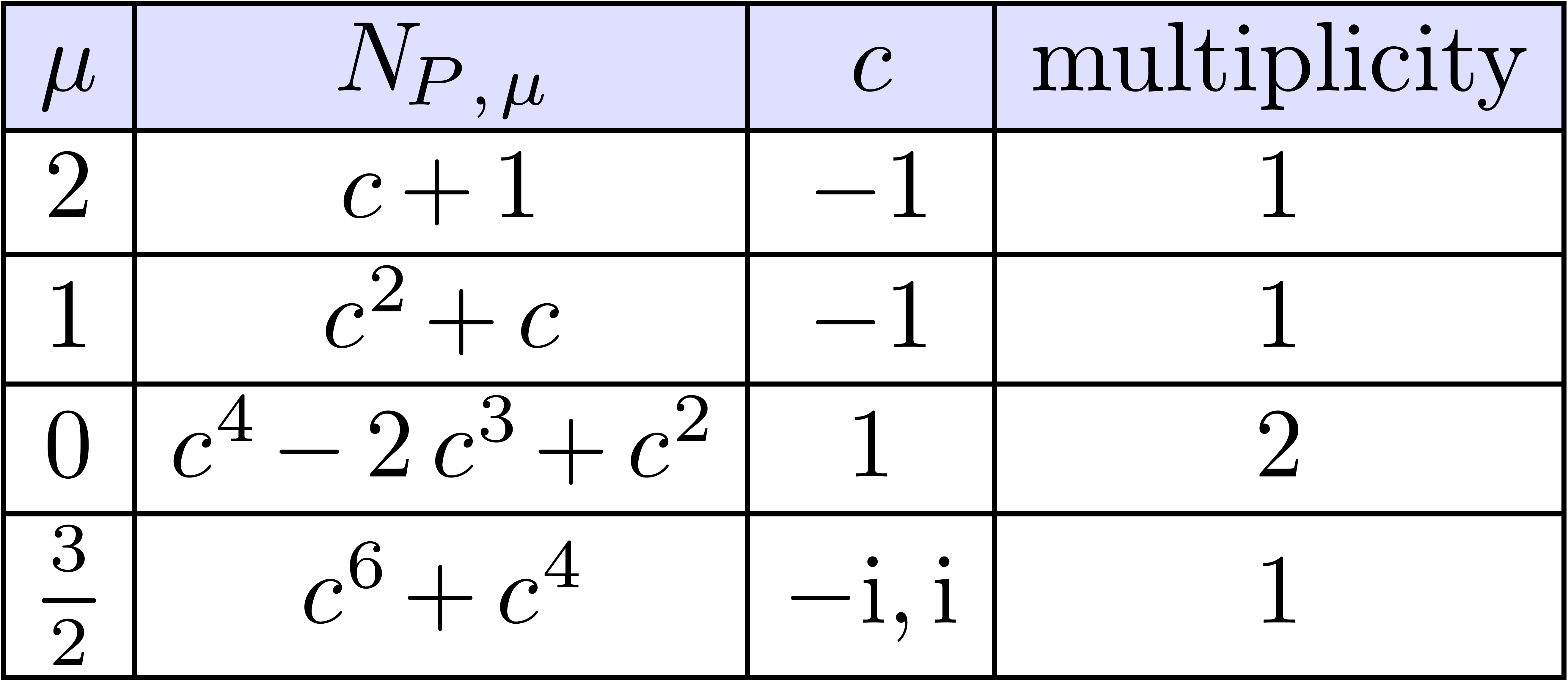
Notice that the Newton polynomials can again be read off from the Newton
polygon. Indeed, when labeling each point  by the
coefficient of in
by the
coefficient of in  ,
the coefficients of are precisely the
coefficients on the edge with slope .
,
the coefficients of are precisely the
coefficients on the edge with slope .
Given a starting term  , we
can now consider the equation
, we
can now consider the equation  which is obtained
from (3.1), by substituting
which is obtained
from (3.1), by substituting  for
, and where
for
, and where  satisfies the asymptotic constraint
  .
For instance, if
.
For instance, if  , then we
obtain:
, then we
obtain:
 |
(3.3) |
The Newton polygon associated to (3.3) is illustrated at the right hand side of figure 3.1. It remains to be shown that we may solve (3.3) by using the same method in a recursive way.
First of all, since the new equation (3.3) comes with the
asymptotic side-condition  ,
it is convenient to study polynomial equations with asymptotic
side-conditions
,
it is convenient to study polynomial equations with asymptotic
side-conditions
 |
(3.4) |
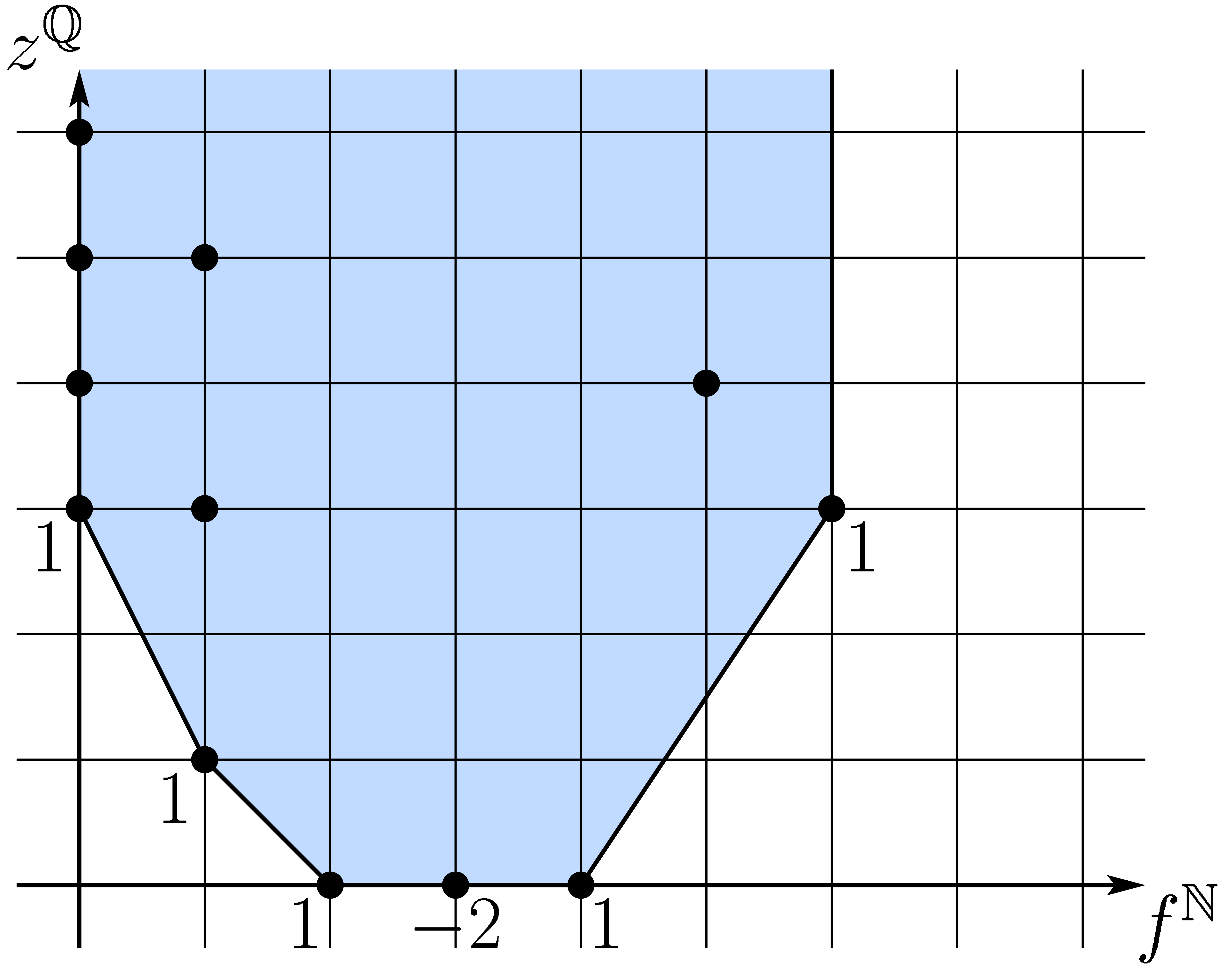  |
Fig. 3.1. The left-hand side shows
the Newton polygon associated to the equation (3.1).
The slopes of the four edges correspond to the starting
exponents 
we obtain the equation (3.3), whose Newton polygon
is shown at the right-hand side. Each non-zero coefficient |
in a systematic way. The case of usual polynomial equations is recovered
by allowing  . In order to
solve (3.4), we now only keep those starting monomials for which satisfy the
asymptotic side condition
. In order to
solve (3.4), we now only keep those starting monomials for which satisfy the
asymptotic side condition  ,
i.e.
,
i.e.  .
.
The highest degree of for a monomial is called the Newton degree of (3.4). If
 , then
is either divisible by (and
, then
is either divisible by (and  is a solution to (3.4)), or (3.4) admits a
starting monomial (and we can carry out one step of the above resolution
procedure). If
is a solution to (3.4)), or (3.4) admits a
starting monomial (and we can carry out one step of the above resolution
procedure). If  , then (3.4) admits no solutions.
Remark 3.1. Graphically speaking, the starting exponents for (3.4) correspond to sufficiently steep slopes in the Newton
polygon (see figure 3.2). Using a substitution  , the equation (3.4) may always be
transformed into an equation
, the equation (3.4) may always be
transformed into an equation

with a normalized asymptotic side-condition (the case  has to be handled with some additional care). Such transformations,
called multiplicative conjugations, will
be useful in chapter 8, and their effect on the Newton
polygon is illustrated in figure 3.2.
has to be handled with some additional care). Such transformations,
called multiplicative conjugations, will
be useful in chapter 8, and their effect on the Newton
polygon is illustrated in figure 3.2.
Given a starting term  or a more general series
 , we next consider the
transformation
, we next consider the
transformation
 |
(3.5) |
with  , which transforms (3.4) into a new asymptotic polynomial equation
 |
(3.6) |
Transformations like (3.5) are called refinements. A refinement is said to be admissible, if the Newton degree of (3.6) does not vanish.
Now the process of computing starting terms and their corresponding
refinements is generally infinite and even transfinite. A
priori, the process therefore only generates an infinite number of
necessary conditions for Puiseux series to
satisfy (3.4). In order to really solve (3.4),
we have to prove that, after a finite number of steps of the Newton
polygon method, and whatever starting terms we chose (when we have a
choice), we obtain an asymptotic polynomial equation with a unique
solution. In the next section, we will prove an implicit function
theorem which guarantees the existence of such a unique solution for
equations of Newton degree one. Such equations will be said to be
quasi-linear.
Returning to our example equation (3.1), it can be checked that each of the refinements

leads to a quasi-linear equation in .
The case

leads to an equation of Newton degree  (it will
be shown later that the Newton degree of (3.6) coincides
with the multiplicity of as a root of ). Therefore, the last case
necessitates one more step of the Newton polygon method:
(it will
be shown later that the Newton degree of (3.6) coincides
with the multiplicity of as a root of ). Therefore, the last case
necessitates one more step of the Newton polygon method:

For both refinements, it can be checked that the asymptotic equation in
 is quasi-linear. Hence, after a finite number of
steps, we have obtained a complete description of the set of solutions
to (3.1). The first terms of these solutions are as
follows:
is quasi-linear. Hence, after a finite number of
steps, we have obtained a complete description of the set of solutions
to (3.1). The first terms of these solutions are as
follows:

Usually the Newton degrees rapidly decreases during refinements and we are quickly left with only quasi-linear equations. However, in the presence of almost multiple roots, the Newton degree may remain bigger than two for quite a while. Consider for instance the equation
 |
(3.7) |
over  , with
  and
and  . This equation has
Newton degree , and after
steps of the ordinary Newton polygon method, we
obtain the equation
. This equation has
Newton degree , and after
steps of the ordinary Newton polygon method, we
obtain the equation

which still has Newton degree .
In order to enforce termination, an additional trick is applied:
consider the first derivative

of the equation (3.7) w.r.t. . This derived equation is quasi-linear, so it
admits a unique solution

Now, instead of performing the usual refinement  in the original equation (3.7), we perform refinement

This yields the equation

Applying one more step of the Newton polygon method yields the admissible refinements

In both cases, we obtain a quasi-linear equation in :

In section 3.3.2, we will show that this trick applies in general, and that the resulting method always yields a complete description of the solution set after a finite number of steps.
Remark 3.2. The idea of using repeated differentiation in order to handle almost multiple solutions is old [Smi75] and has been used in computer algebra before [Chi86, Gri91]. Our contribution has been to incorporate it directly into the Newton polygon process, as will be shown in more detail in section 3.3.2.
In the previous section, we have stressed the particular importance of quasi-linear equations when solving asymptotic polynomial equations. In this section, we will prove an implicit series theorem for polynomial equations. In the next section, we will apply this theorem to show that quasi-linear equations admit unique solutions. The implicit series theorem admits several proofs (see the exercises). The proof we present here uses a powerful syntactic technique, which will be generalized in chapter 6.
Theorem 3.3. Let
be a ring and a monomial monoid. Consider the
polynomial equation
 |
(3.8) |
with coefficients  , such
that
, such
that  and
and  .
Then
.
Then  .
.
Proof. Since , the
series  is invertible in
  . Modulo division of (3.20) by , we may therefore assume without
loss of generality that
. Modulo division of (3.20) by , we may therefore assume without
loss of generality that  .
Setting
.
Setting  for all
  ,
we may then rewrite (3.20) as
,
we may then rewrite (3.20) as
 |
(3.9) |
Now consider the set  of trees with nodes of
arities in
of trees with nodes of
arities in  and such that each node of arity is labeled by a monomial in
  . To each such tree

we recursively associate a coefficient  and a
monomial
and a
monomial  by
by

Now we observe that each of these monomials  is
infinitesimal, with
is
infinitesimal, with
 |
(3.10) |
Hence the mapping  is strictly increasing, when
is given the embeddability ordering from section
1.4. From Kruskal's theorem, it follows that the family
is strictly increasing, when
is given the embeddability ordering from section
1.4. From Kruskal's theorem, it follows that the family
 is well-based and even grid-based, because of
(3.10). We claim that
is well-based and even grid-based, because of
(3.10). We claim that  is the unique
solution to (3.9).
is the unique
solution to (3.9).
First of all, is indeed a solution to (3.9),
since

In order to see that is the unique solution to
(3.20), consider the polynomial  . Since
  ,
we have
,
we have  for all ,
whence in particular
for all ,
whence in particular  .
Furthermore, implies
.
Furthermore, implies  . Now assume that
  were
another root of . Then
were
another root of . Then  would be a root of ,
so that
would be a root of ,
so that
 |
(3.11) |
since  is invertible.

where  is a grid-based family with
and .
is a grid-based family with
and .
Exercise 3.2. Give an alternative proof
of theorem 3.3, using the fact that (3.9)
admits a unique power series solution in  ,
when considered as an equation with coefficients in
,
when considered as an equation with coefficients in  .
.
Exercise 3.3. Assuming that is totally ordered, give yet another alternative proof
of theorem 3.3, by computing the terms of the unique
solution by transfinite induction.
Exercise 3.4. Let  denote the ring of non-commutative power series in
  over . Consider the
equation
over . Consider the
equation
 |
(3.12) |
with  ,
,  and invertible
  .
Prove that (3.12) admits a unique infinitesimal solution
.
Prove that (3.12) admits a unique infinitesimal solution
 .
.
Let be a constant field of characteristic zero
and a totally ordered monomial group with -powers. Consider the
asymptotic polynomial equation
 |
(3.13) |
with coefficients in and . In order to capture ordinary polynomial equations,
we will also allow  , where
 is a formal monomial with
  . A starting monomial
of relative to (3.13) is a monomial
. A starting monomial
of relative to (3.13) is a monomial
 in ,
such that there exist
in ,
such that there exist  and
and  with
with  and
and  for all other
 . To such a starting monomial
we associate the equation
. To such a starting monomial
we associate the equation
 |
(3.14) |
and  is called the Newton polynomial associated to .
A starting term of
relative to (3.13) is a term
is called the Newton polynomial associated to .
A starting term of
relative to (3.13) is a term  ,
where is a starting monomial of
relative to (3.13) and
,
where is a starting monomial of
relative to (3.13) and  a non-zero
root of
a non-zero
root of  . In that case, the
multiplicity of
. In that case, the
multiplicity of  is defined to be the multiplicity of
as a root of . Notice that
there are only a finite number of starting terms relative to (3.13).
is defined to be the multiplicity of
as a root of . Notice that
there are only a finite number of starting terms relative to (3.13).
Proposition 3.4. Let
be a non-zero solution to is a starting term for
The Newton degree  of (3.13) is defined to be the largest degree of the Newton
polynomial associated to a monomial .
In particular, if there exists no starting monomial relative to (3.13), then the Newton degree equals the valuation of in . If
of (3.13) is defined to be the largest degree of the Newton
polynomial associated to a monomial .
In particular, if there exists no starting monomial relative to (3.13), then the Newton degree equals the valuation of in . If
 , then we say that (3.13)
is quasi-linear. The previous proposition
implies that (3.13) does not admit any solution, if .
, then we say that (3.13)
is quasi-linear. The previous proposition
implies that (3.13) does not admit any solution, if .
Lemma 3.5. If .
Proof. If  , then our
statement follows from proposition 3.4, since there are no
starting monomials. Otherwise, our statement follows from theorem 3.3, after substitution of
, then our
statement follows from proposition 3.4, since there are no
starting monomials. Otherwise, our statement follows from theorem 3.3, after substitution of  for in (3.13), where
  is chosen -maximal such that
 for all ,
and after division of (3.13) by
for all ,
and after division of (3.13) by  .
.
A refinement is a change of variables together with the imposition of an asymptotic constraint:
 |
(3.15) |
where  and
and  .
Such a refinement transforms (3.13) into an asymptotic
polynomial equation in :
.
Such a refinement transforms (3.13) into an asymptotic
polynomial equation in :
 |
(3.16) |
where
 |
(3.17) |
for each . We say that the
refinement (3.15) is admissible
if the Newton degree of (3.16) is strictly positive.
Lemma 3.6. Consider the refinement  .
Then
.
Then
Proof. Let  be maximal such that
  for all , and
denote
for all , and
denote  . Then is bounded by the Newton degree of (3.13) and

for all . In particular,
denoting the multiplicity of  as a root of by
  , we
have
, we
have  . Moreover, for all
 , we have
  . Hence, for any
  and
and
 , we have
  . This shows that the Newton degree of (3.16) is at most .
Let us now show that the Newton degree of . Choose  large enough, so that

for all  . Then
  .
.
If one step of the Newton polygon method does not suffice to decrease the Newton degree, then two steps do, when applying the trick from the next lemma:
Lemma 3.7. Let be
the Newton degree of admits a unique starting monomial  and a unique root of
multiplicity , then
and a unique root of
multiplicity , then
The equation
 |
(3.18) |
is quasi-linear and its unique solution satisfies  .
.
The Newton degree of any refinement

relative to  is strictly inferior to .
Proof. Notice first that  for all
polynomials and monomials . Consequently, (3.18) is quasi-linear
and is a single root of
for all
polynomials and monomials . Consequently, (3.18) is quasi-linear
and is a single root of  . This proves (a).
As to (b), we first observe that  .
Given
.
Given  , it follows that
  . In particular, there do not exist
 with
with  .
In other words,
.
In other words,  does not admit roots of
multiplicity . We conclude by
lemma 3.6.
does not admit roots of
multiplicity . We conclude by
lemma 3.6.
Theorem 3.8. Let
be an algebraically closed field of characteristic zero and a totally ordered monomial group with -powers. Then is
algebraically closed.
Proof. Consider the following algorithm:
Algorithm polynomial_solve
Input:
An asymptotic polynomial equation (3.13).
Output:
The set of solutions to (3.13).
Compute the starting terms  of relative to (3.13).
If  and
and  is a root of
multiplicity of
is a root of
multiplicity of  , then let be the unique
solution to (3.18). Refine (3.15) and
apply polynomial_solve to (3.16). Return the
so obtained solutions to (3.13).
, then let be the unique
solution to (3.18). Refine (3.15) and
apply polynomial_solve to (3.16). Return the
so obtained solutions to (3.13).
For each  , refine

and apply polynomial_solve to the new equation in . Collect and return the so
obtained solutions to (3.13), together with , if is
divisible by .
The correctness of polynomial_solve is clear; its termination
follows from lemmas 3.6(b) and 3.7(b).
Since is algebraically closed, all Newton
polynomials considered in the algorithm split over . Hence, polynomial_solve returns solutions to (3.13) in , when counting with multiplicities. In
particular, when taking  , we
obtain solutions, so is
algebraically closed.
, we
obtain solutions, so is
algebraically closed.
Corollary 3.9. Let
be a real closed field and a totally ordered
monomial group with -powers.
Then is real closed.
Proof. By the theorem, a polynomial equation  of degree over admits
solutions in
of degree over admits
solutions in  ,
when counting with multiplicities. Moreover, each root
,
when counting with multiplicities. Moreover, each root  is imaginary, because

for such . Therefore all real
roots of are in .
Corollary 3.10. The field of Puiseux series over an algebraically resp. real closed
field is algebraically resp. real closed.
Exercise 3.5. Consider an asymptotic
algebraic equation (3.13) of Newton degree . Let  be the starting
terms of (3.13), with multiplicities
be the starting
terms of (3.13), with multiplicities  . Prove that

Also show that  if is algebraically closed.
Exercise 3.6.
Show that the computation of all solutions to (3.13) can be represented by a finite tree, whose non-root nodes are labeled by refinements. Applied to (3.1), this would yields the following tree:

Show that the successors of each node may be ordered in a natural
way, if is a real field, and if we
restrict our attention to real algebraic solutions. Prove that the
natural ordering on the leaves, which is induced by this ordering,
corresponds to the usual ordering of the solutions.
Exercise 3.7.
Generalize the results of this chapter to asymptotic equations of
infinite degree in ,
but of finite Newton degree.
Give an example of an asymptotic equation of infinite degree in
, with infinitely many
solutions.
Exercise 3.8. Consider an asymptotic polynomial equation

of Newton degree ,
with  and
and  .
Consider the monomial monoid
.
Consider the monomial monoid  with
with

Show that there exists a unique invertible series  such that
  is a monoic polynomial in
  .
.
Show that  .
.
In this section, we show that grid-based series may be represented by (finite sums of) multivariate Laurent series in which we substitute an infinitesimal monomial for each variable. Such representations are very useful for finer computations with grid-based series.
Let be a grid-based algebra. A Cartesian
representation for a series
is a multivariate Laurent series  ,
such that
,
such that  for some morphism of monomial monoids
 . Writing
  , with
  ,
we may also interpret as the product of a
“series”
,
we may also interpret as the product of a
“series”  in
in  and the monomial
  .
.
More generally, a semi-Cartesian representation for is an expression of the form

where  ,
,  and
and  is a morphism of monomial monoids.
Any grid-based series admits a
semi-Cartesian representation.
If is a monomial group, which is generated
by its infinitesimal elements, then each grid-based series admits a Cartesian representation.
Proof.
Let  and
and  be such
that
be such
that

For each  , let
, let

Let

for all  and let
  .
Then
.
Then

For certain  and
and  , we may write

for all . Let  and
and

Then  .
.
Cartesian or semi-Cartesian representations  and
and
 are said to be compatible, if
  and
and  belong
to the same algebra
belong
to the same algebra  of Laurent series, and if
 .
.
Any  admit compatible semi-Cartesian
representations.
admit compatible semi-Cartesian
representations.
If is a monomial group, which is generated
by its infinitesimal elements, then any
admit compatible Cartesian representations.
Proof. By the previous proposition,  admit
semi-Cartesian representations
admit
semi-Cartesian representations  ,
where
,
where  and
and  for each . Now consider

Then  for each ,
where
for each ,
where  is the image of
  under the natural inclusion of
  into
into  . This proves (a); part (b) is
proved in a similar way.
. This proves (a); part (b) is
proved in a similar way.
In proposition 3.12 we drastically increased the size of the Cartesian basis in order to obtain compatible Cartesian representations. The following lemma is often useful, if one wants to keep this size as low as possible.
Lemma 3.13. Let  be infinitesimal elements of a totally ordered monomial group with -powers,
such that
be infinitesimal elements of a totally ordered monomial group with -powers,
such that  . Then there exist
infinitesimal
. Then there exist
infinitesimal  with
with  .
.
Proof. It suffices to prove the lemma for  ; the general case follows by induction over . The case
is proved by induction over .
For
; the general case follows by induction over . The case
is proved by induction over .
For  , there is nothing to
prove. So assume that
, there is nothing to
prove. So assume that  and let
  with
with  . Without loss of
generality, we may assume that
. Without loss of
generality, we may assume that  ,
modulo a permutation of variables. Putting
,
modulo a permutation of variables. Putting  ,
we now distinguish the following three cases:
,
we now distinguish the following three cases:
If , then there exist
infinitesimal  , such that
 , by the induction
hypothesis. Taking
, by the induction
hypothesis. Taking  , we
now have
, we
now have  , since .
If  , then
  , and we may take
  .
.
If  , then there exists
infinitesimal , such that
, then there exists
infinitesimal , such that
 . Taking
  , we again have
  .
.
When doing computations on grid-based series in , one often works with respect to a Cartesian
basis  of
infinitesimal elements in .
Each time one encounters a series which cannot
be represented by a series in
of
infinitesimal elements in .
Each time one encounters a series which cannot
be represented by a series in  ,
one has to replace
,
one has to replace  by a wider
Cartesian basis
by a wider
Cartesian basis  with
with  . The corresponding mapping
  is called a widening. Lemma 3.13
enables us to keep the Cartesian basis reasonably small during the
computation.
is called a widening. Lemma 3.13
enables us to keep the Cartesian basis reasonably small during the
computation.
Let be a ring and a
monomial group which is generated by its infinitesimal elements. Given a
set  for each
  ,
we denote by
,
we denote by  the set of all
grid-based series , which
admit a Cartesian representation
the set of all
grid-based series , which
admit a Cartesian representation  for some
  . In this section, we will show
that if the
. In this section, we will show
that if the  satisfy appropriate conditions, then
many types of computations which can be carried out in
can also be carried out in .
satisfy appropriate conditions, then
many types of computations which can be carried out in
can also be carried out in .
Let be a ring. A sequence  with is said to be a Cartesian
community over ,
if the following conditions are satisfied:
with is said to be a Cartesian
community over ,
if the following conditions are satisfied:
 .
.
is a
-algebra
for each
 .
.
are stable under strong monomial morphisms.
In CC3, a strong monomial morphism is strong -algebra
morphism which maps monomials to monomials. In our case, a monomial
preserving strong morphism from  into
into  is always of the form

where  and
and  for all . In particular, CA3 implies
that the are stable under widenings.
for all . In particular, CA3 implies
that the are stable under widenings.
Proposition 3.14. Let be a
Cartesian community over and let be a monomial group. Then is a
-algebra.
Proof. We clearly have  .
Let
.
Let  . Mimicking the proof of
proposition 3.12, we observe that
and
. Mimicking the proof of
proposition 3.12, we observe that
and  admit compatible Cartesian representations
 . Then ,
  and
are Cartesian representations of
and
are Cartesian representations of  ,
,
 resp.
resp.  .
.
A local community is a Cartesian community , which satisfies the following
additional conditions:
 with
with
 ,
we have
,
we have
 .
.
 and
and
 ,
we have
,
we have
 .
.
 with
with
 and
and
 ,
the unique series
,
the unique series
 with
with
 belongs to
.
belongs to
.
In LC1 and LC3, the notation  stands for the coefficient of
  in
. The condition LC3
should be considered as an implicit function theorem for the local
community. Notice that is stable under
in
. The condition LC3
should be considered as an implicit function theorem for the local
community. Notice that is stable under  for all {
 },
since
},
since
 |
(3.19) |
Remark 3.15. In [vdH97], the conditions
LC2 and LC3 were replaced by a single,
equivalent condition: given as in
LC3, we required that  ,
for the unique strong -algebra
morphism
,
for the unique strong -algebra
morphism  , such that
  and
and  . We
also explicitly requested the stability under differentiation, although
(3.19) shows that this is superfluous.
. We
also explicitly requested the stability under differentiation, although
(3.19) shows that this is superfluous.
Example 3.16. Let be a subfield of  and let
  be the set of
convergent power series in variables over , for each . Then the form a local
community. If is a monomial group, then
be the set of
convergent power series in variables over , for each . Then the form a local
community. If is a monomial group, then  will also be called the set of
convergent grid-based series
in over .
will also be called the set of
convergent grid-based series
in over .
Example 3.17. For each ,
let be the set of power series in  , which satisfy an algebraic equation over
 . Then the
form a local community.
. Then the
form a local community.
In this and the next section,  is a local
community. A Cartesian representation
is a local
community. A Cartesian representation  is said to
be faithful, if for each
dominant monomial of , there exists a dominant monomial
is said to
be faithful, if for each
dominant monomial of , there exists a dominant monomial  of , with
  .
.
Proposition 3.18. Let  be a
local community and .
Then
be a
local community and .
Then
For each  and
and  ,
we have
,
we have  .
.
For each initial segment  ,
we have
,
we have

Proof. For each  , let
, let
 . We will prove (a) by
a weak induction over . If
. We will prove (a) by
a weak induction over . If
 , then
  . If
. If  ,
then
,
then

By the weak induction hypothesis and LC1, we thus have  .
.
In order to prove (b), let  be the
finite anti-chain of maximal elements of
be the
finite anti-chain of maximal elements of  ,
so that
,
so that  . Let be the number of variables which effectively occur in
 , i.e. the
number of
, i.e. the
number of  , such that
  with
with  for some
  . We prove (b) by weak induction over
. If , then either
. We prove (b) by weak induction over
. If , then either  and
and  , or ,
 and
and  .
.
Assume now that and order the variables  in such a way that
  effectively occurs in one of the
  .
For each
.
For each  , let
, let

We observe that

In particular, if  is maximal with
  , then
  for all
  and
and

so that

Moreover, for each , at most
variables effectively occur in the set  of dominant monomials of
  .
Therefore
.
Therefore  , by the induction
hypothesis.
, by the induction
hypothesis.
Proposition 3.19. Given a Cartesian representation

of a series  , its
truncation
, its
truncation

is a faithful Cartesian representation of the same series  .
.
Proposition 3.20. Let  be series, which is either
infinitesimal,
bounded, or
regular.
Then admits a Cartesian representation in
 for some ,
which is also infinitesimal, bounded resp. regular.
for some ,
which is also infinitesimal, bounded resp. regular.
Proof. Assume that is infinitesimal and
let  be a faithful Cartesian representation of
, with dominant monomials
be a faithful Cartesian representation of
, with dominant monomials
 . For each
  , let
, let

with  . Then
  and
and

is an infinitesimal Cartesian representation of
in  , when setting
  for each . This
proves (a).
for each . This
proves (a).
If is bounded, then let
be an infinitesimal Cartesian representation of  . Now
. Now  is a bounded Cartesian
representation of . This
proves (b).
is a bounded Cartesian
representation of . This
proves (b).
Assume finally that  is regular, with dominant
monomial
is regular, with dominant
monomial  . Let be a bounded Cartesian representation of
  . Since
  ,
the series is necessarily regular. Now take a
Cartesian monomial
,
the series is necessarily regular. Now take a
Cartesian monomial  which represents (e.g. among the dominant monomials of a faithful Cartesian
representation of ). Then
which represents (e.g. among the dominant monomials of a faithful Cartesian
representation of ). Then
 is a regular Cartesian representation of .
Theorem 3.21. Let
be a local community over a ring and let be a monomial monoid. Consider the polynomial
equation
 |
(3.20) |
with coefficients  , such
that
, such
that  and
and  .
Then
.
Then  .
.
Proof. By proposition 3.20, there exist bounded
Cartesian representations  for certain
  . Now consider the series

We have  and
and  ,
so there exists a with
,
so there exists a with

by LC3. We conclude that
satisfies  . The uniqueness of
follows from theorem 3.3.
. The uniqueness of
follows from theorem 3.3.
Theorem 3.22. Let
be a local community over a (real) algebraically closed field and a totally ordered monomial
group with -powers. Then is a (real) algebraically closed field.
Proof. The proof is analogous to the proof of theorem 3.8.
In the present case, theorem 3.21 ensures that  in step 2 of polynomial_solve.
Exercise 3.9. Let
be a ring, a monomial monoid and a local community. We define to
be the set of series in , which admit a semi-Cartesian
representation

with  for some , and
  . Which results from this section generalize
to this more general setting?
. Which results from this section generalize
to this more general setting?
Exercise 3.10. Let
be a field. A series in
is said to be differentially algebraic, if the
field generated by its partial derivatives  has
finite transcendence degree over .
Prove that the collection of such series forms a local community over
.
has
finite transcendence degree over .
Prove that the collection of such series forms a local community over
.
Exercise 3.11. Assume that is an effective field, i.e. all field
operations can be performed by algorithm. In what follows, we will
measure the complexity of algorithms in terms of the number of such
field operations.
A series  is said to be
effective, if there is an algorithm which
takes
is said to be
effective, if there is an algorithm which
takes  on input, and which outputs
  . Show that the collection of
effective series form a local community.
. Show that the collection of
effective series form a local community.
An effective series is said to be of
polynomial time complexity, if there is an algorithm,
which takes  on input and which computes
 for all
  with
with  in time
  .
Show that the collection of such series forms a local community.
What about even better time complexities?
.
Show that the collection of such series forms a local community.
What about even better time complexities?
Exercise 3.12. Let
be a local community and let
be a Cartesian representation of an infinitesimal,
bounded or regular grid-based series in . Show that, modulo widenings,
there exists an infinitesimal, bounded resp. regular Cartesian
representation of , with
respect to a Cartesian basis with at most
elements.
If  and
and  ,
then show that
,
then show that  .
.
If is totally ordered, then prove that
is a field.
Exercise 3.14. Let be a local community over a field
and let be a totally ordered monomial group.
Prove that  for any
  , and
, and

Exercise 3.15. Let
be a Cartesian community. Given monomial groups
and , let  be the set of strong -algebra
morphisms from into
and
be the set of strong -algebra
morphisms from into
and  the set of
  ,
such that
,
such that  for all .
Given  and
and  ,
where
,
where  is a third monomial group, prove
that
is a third monomial group, prove
that  .
.
Given and  such
that
such
that  , prove that
  .
.
Exercise 3.16. Let be a subfield of and let and be monomial groups with
 . Prove that
  . Does this property generalize to other
local communities?
. Does this property generalize to other
local communities?
Exercise 3.17. Let
be the local community from example 3.17 and let be a totally ordered monomial group. Prove that
is isomorphic to the algebraic closure of
.
Exercise 3.18. Does theorem 3.22 still hold if we remove condition LC2 in the definition of local communities?
Exercise 3.19. Consider the resolution
of  , with
  and .
and .
Given a starting term  of multiplicity
, let
of multiplicity
, let  be minimal for such that
  for all . Show that
there exist Cartesian coordinates
for all . Show that
there exist Cartesian coordinates  with
with
 , in which
  admits a bounded Cartesian representations
  for all
  .
.
Consider a bounded Cartesian representation  with
with  and let
  .
Given
.
Given  , let
, let

Show that  is a series in
  .
.
For each  , let
, let  be initial segment generated by the
  such that
  ,
and
,
and  its complement. We say that
  is the part of multiplicity
  of as a zero of
  . Show that
  can be
determined effectively for all .
can be
determined effectively for all .
In polynomial_solve, show that refinements of the type

where  is the unique solution to
  , may be replaced by
refinements
, may be replaced by
refinements

Let be a totally ordered exp-log field. This
means that is a totally ordered field with an
exponential function and a partial logarithmic function which satisfies
similar properties as those defined on the real numbers. Axioms for
exp-log fields will be given in section 4.1. For the
moment, the reader may assume that .
The aim of this chapter is the construction of the totally ordered
exp-log field  of grid-based transseries in over .
This means that is a field of grid-based series
with an additional exponential structure. Furthermore,
contains as an infinitely large monomial.
Actually, the field carries much more structure:
in the next chapter, we will show how to differentiate, integrate,
compose and invert transseries. From corollary 3.9, it also
follows that is real closed. In chapter 9,
this theorem will be generalized to algebraic differential equations.
of grid-based transseries in over .
This means that is a field of grid-based series
with an additional exponential structure. Furthermore,
contains as an infinitely large monomial.
Actually, the field carries much more structure:
in the next chapter, we will show how to differentiate, integrate,
compose and invert transseries. From corollary 3.9, it also
follows that is real closed. In chapter 9,
this theorem will be generalized to algebraic differential equations.
As to the construction of ,
let us first consider the field  .
Given an infinitesimal series ,
we may naturally define
.
Given an infinitesimal series ,
we may naturally define

Using the exp-log structure of ,
these definitions may be extended to  for
for  and to
  for
for  . However, nor the logarithm of , nor the exponential of any infinitely large
series are defined. Consequently, we have to add
new monomials to
. However, nor the logarithm of , nor the exponential of any infinitely large
series are defined. Consequently, we have to add
new monomials to  in order to obtain a field of
grid-based series which is stable under exponentiation and logarithm.
in order to obtain a field of
grid-based series which is stable under exponentiation and logarithm.
Now it is easy to construct a field of grid-based series  which is stable under logarithm (in the sense that
  is defined for all strictly positive ). Indeed, taking
  ,
we set
,
we set

for monomials  (here
(here  stands for the -th
iterated logarithm). For general
stands for the -th
iterated logarithm). For general  ,
we define
,
we define

where  as above.
In order to construct a field  of grid-based
series with an exponentiation, we first have to decide what monomial
group to take. The idea is to always take
exponentials of purely infinite series for the monomials in . For instance,
of grid-based
series with an exponentiation, we first have to decide what monomial
group to take. The idea is to always take
exponentials of purely infinite series for the monomials in . For instance,  is a
monomial. On the other hand,
is a
monomial. On the other hand,  is not a monomial
and we may expand it in terms of using
is not a monomial
and we may expand it in terms of using

More generally, as soon as each purely infinite series in admits an exponential, then is
closed under exponentiation: for all  we take

with  as above.
In section 4.2, we first study abstract fields of
transseries. These are totally ordered fields of grid-based series, with
logarithmic functions that satisfy some natural compatibility conditions
with the serial structures. Most of these conditions were briefly
motivated above. In section 4.3 we construct the field of transseries in .
We start with the construction of the field of
logarithmic transseries. Next, we close this field under exponentiation
by repeatedly inserting exponentials of purely infinite series as new
monomials. In section 4.4, we prove the incomplete
transbasis theorem, which provides a convenient way to represent and
compute with grid-based transseries.
A partial exponential ring is
a ring with a partial exponential
function  ,
such that
,
such that
 .
.
 ,
for all
,
for all
 .
.
The second condition stipulates in particular that  , whenever
  .
If
.
If  , then we say that is an exponential ring.
If is an exponential function, then we will also
write
, then we say that is an exponential ring.
If is an exponential function, then we will also
write  for
for  and
and  for the -th
iterate of (i.e.
for the -th
iterate of (i.e.  and
and  for all
  ).
).
The field of real numbers is a classical example
of an exponential field. Moreover, the real numbers carry an ordering
and it is natural to search for axioms which model the compatibility of
the exponential function with this ordering. Unfortunately, an explicit
set of axioms which imply all relations satisfied by the exponential
function on has not been found yet.
Nevertheless, Dahn and Wolter have proposed a good candidate set of
axioms [DW84].
We will now propose a similar system of axioms in the partial context.
For each , we denote the
Taylor expansion of at order
by

We also denote

so that  . An ordered
partial exponential ring
is a partially ordered ring ,
with a partial exponential function
. An ordered
partial exponential ring
is a partially ordered ring ,
with a partial exponential function  ,
which satisfies E1, E2 and
,
which satisfies E1, E2 and
 ,
for all
,
for all
 and
.
and
.
If , then we say that is an ordered exponential ring.
Proposition 4.1. Let be an
ordered ring in which  . Given
a partial exponential function on which
satisfies
. Given
a partial exponential function on which
satisfies

for all and .
Proof. Assume that  .
We cannot have
.
We cannot have  , since
otherwise
, since
otherwise

If  , then

whence  .
.
Proposition 4.2. is a
totally ordered exponential field.
Proof. Let . For  , we have

For  , we have shown above
that
, we have shown above
that  .
.
Proposition 4.3. Let
be an ordered partial exponential ring. Then
is injective.
 , for all
  .
.
If  is a -module,
then
is a -module,
then

Proof. Assume that  ,
for some
,
for some  . Then

and similarly  . Hence,

so that both  and
and  .
This proves that
.
This proves that  , whence
 is injective.
Assume now that  for some . Then

Consequently,

and  , by the injectivity of
. Inversely, assume that
, by the injectivity of
. Inversely, assume that  for some .
Then
for some .
Then

whence . We again conclude
that , since  . This proves (b).
If , then (c)
follows from (b). If ,
then  implies

for all  .
.
Instead of axiomatizing partial exponential functions on a ring, it is also possible to axiomatize partial logarithmic functions. The natural counterparts of E1, E2 and E3 are
 .
.
 ,
for all
,
for all
 .
.
 ,
for all
,
for all
 and
.
and
.
Notice that the second condition assumes the existence of a partial
inversion  , whose domain
contains
, whose domain
contains  . The -th iterate of will be
denoted by
. The -th iterate of will be
denoted by  .
.
In a similar fashion, we define a partial logarithmic ring to be a ring
with a partial logarithmic function which
satisfies L1 and L2. An ordered partial logarithmic ring
is an ordered ring with a partial logarithmic
function which satisfies L1, L2 and L3. In the case
when  for such a ring, then we say that is an ordered logarithmic ring.
Proposition 4.4.
Let be a partial exponential ring, such
that is injective. Then the partial
inverse of
satisfies
If is an ordered partial exponential ring,
then is injective, and its partial inverse
satisfies
Let be a partial logarithmic ring, such
that is injective. Then the partial
inverse of
satisfies
If is an ordered partial logarithmic ring,
then is injective, and its partial inverse
satisfies
Proof. Let be a partial exponential ring,
such that is injective. Then we clearly have
L1. Now assume that  .
Then
.
Then  , whence
  . Furthermore, if
  ,
then
,
then  , so that
  . Consequently,
  and
and
 . This proves L2 and
(a). As to (b), if is an ordered
partial exp-log ring, then is injective by
proposition 4.3(a). The property L3 directly
follows from E3.
. This proves L2 and
(a). As to (b), if is an ordered
partial exp-log ring, then is injective by
proposition 4.3(a). The property L3 directly
follows from E3.
Assume now that is a partial logarithmic ring,
such that  is injective. We clearly have
E1. Given
is injective. We clearly have
E1. Given  and
and  in
in
 , we have
  and in particular
  . It
follows that
. It
follows that  . This proves
E2 and (c).
. This proves
E2 and (c).
Assume finally that is an ordered partial
logarithmic ring. Let be such that  . Then

Hence  , since
  . Similarly,
  and , which proves that
  is injective. The property E3 directly follows from
L3.
is injective. The property E3 directly follows from
L3.
If (a) and (c) (resp. (b) and (d)) are
satisfied in the above proposition, then we say that
is a partial exp-log ring
(resp. an ordered partial exp-log ring). An ordered exp-log
ring is an ordered partial exp-log
ring , such that and  . An
ordered (partial) exponential, logarithmic resp. exp-log ring, which is
also an ordered field is called an ordered (partial) exponential,
logarithmic resp. exp-log field.
In a partial exp-log ring, we extend the notations
and to the case when , by setting
. An
ordered (partial) exponential, logarithmic resp. exp-log ring, which is
also an ordered field is called an ordered (partial) exponential,
logarithmic resp. exp-log field.
In a partial exp-log ring, we extend the notations
and to the case when , by setting  and
and  , if
, if  .
.
Assume now that is a ring with -powers, for some subring  . An exponential resp. logarithmic function is
said to be compatible with the -powers
structure on if
. An exponential resp. logarithmic function is
said to be compatible with the -powers
structure on if
 ,
for all
,
for all
 and
;
resp.
and
;
resp.
 ,
for all
and
.
,
for all
and
.
Here we understand that  in E4 and
  in L4. Notice that E4 and L4 are
equivalent, if and are
partial inverses. Notice also that any totally ordered exp-log field
naturally has -powers:
set
in L4. Notice that E4 and L4 are
equivalent, if and are
partial inverses. Notice also that any totally ordered exp-log field
naturally has -powers:
set  for all
  and
and  .
.
Exercise 4.1. Let
be an exponential ring. Show that for all  , we have
  .
.
Exercise 4.2. Show that the only
exponential function on the totally ordered field of real numbers is the usual exponential function.
Exercise 4.3. Let
be a totally ordered exponential field. Show that the exponential
function on is continuous. That is, for all
and  in , there exists a
  , such that
  ,
for all
,
for all  with
with  .
Show also that the exponential function is equal to its own
derivative.
.
Show also that the exponential function is equal to its own
derivative.
Exercise 4.4. Let
be an ordered partial exponential ring. Given
and , prove that
 , if
, if  .
.
 , if
, if  .
.
Let be a totally ordered exp-log field, a totally ordered monomial group with -powers. Assume that we have a partial
logarithmic function on the totally ordered field  with -powers. We say that
is a field of grid-based
transseries (or a field of
transseries) if
with -powers. We say that
is a field of grid-based
transseries (or a field of
transseries) if
 .
.
 ,
for all
,
for all
 .
.
 ,
for all
,
for all
 ,
where
,
where
 .
.
Intuitively speaking, the above conditions express a strong
compatibility between the logarithmic and the serial structure of .
Example 4.5. Assume that  is a
field of transseries, such that
is a
field of transseries, such that  ,
and such that is stable under exponentiation.
Then
,
and such that is stable under exponentiation.
Then  is a monomial in
  . The series
  is not a
monomial, since
is not a
monomial, since  . We have

On the other hand,  is a monomial, since

Proposition 4.6. Let
be a field of transseries. Then
Given  , the canonical
decomposition of is given by
, the canonical
decomposition of is given by

Given  , we have

Given  , we have

For all  , we have
  ,
,  and
and
 .
.
Proof.
Follows from L1, L2, T2 and T3.
We have

The other relations are proved in a similar way.
We have

The other relations are proved similarly.
Let . Then  , by (b), whence
  . Furthermore,

Consequently,  , since
  . It follows that

Since is total on , we infer that  .
Therefore, . Finally,
.
Therefore, . Finally,  and (c) imply that
by (c).
and (c) imply that
by (c).
The following lemma, which is somehow the inverse of proposition 4.6(a) and (d), will be useful for the construction of fields of transseries.
Lemma 4.7. Let be
a partial function on , which
satisfies
 , for all
  and
and  .
.
 , for all .
 , for all
  .
.
Then is a logarithmic function, which is
compatible with the ordering and -powers
on . Hence,
is a field of grid-based transseries.
Proof. We clearly have L1. Given , we also have

Here

by proposition 2.18 and the fact that  in . This proves L2.
Let us now show that

for all  and .
Assume first that
and .
Assume first that  . If
. If  , then we have

Otherwise,  and
and

If , then  . Consequently,

If  , let us show that
  , for all , which clearly implies that
  . We first observe that
  for
all
for
all  , since
  and
and  . Furthermore,
  , for all . Taking
  ,
we get
,
we get  . This proves
L3.
. This proves
L3.
Let us finally show that for any and . Denoting
 , we have

Indeed, proposition 2.18 implies that  , since
  is a formal
identity in
is a formal
identity in  .
.
Exercise 4.5. Let
be a field of transseries.
Show that  for all
  , where
  .
.
For each  , show that

For each  , show that
 ,
,  and
and  .
.
Exercise 4.6. Let  ,
,  and
and  be as above. Prove the following formal identities:
 ;
;
;
 ;
;
.
Hint: prove that the left and right hands sides satisfy the same (partial) differential equations and the same initial conditions.
Let be a fixed totally ordered exp-log field,
such as , and a formal infinitely large variable. In this section, we
will construct the field of
grid-based transseries in over . We proceed as follows:
We first construct the field

of logarithmic transseries in .
Given a field of transseries ,
we next show how to construct its exponential extension  : this is the smallest field of transseries
with
: this is the smallest field of transseries
with  and such that
  is defined in
  for all
  .
.
We finally consider the sequence

of successive exponential extensions of . Their union

is the desired field of grid-based transseries in
over .

Given a monomial  , we define
 by
by

We extend this definition to  ,
by setting
,
by setting

for each . Here we recall
that .
Proposition 4.8.  is a field of transseries.
Proof. Clearly, , for
all  and .
Now let
and .
Now let  . Then
  , for certain
  with
with
 . Hence,
  , since
  and
and  . Now the proposition follows from
lemma 4.7.
. Now the proposition follows from
lemma 4.7.
Let be a field of transseries and let

be the monomial group of formal exponentials
with  , which is isomorphic to
the totally ordered -module
, which is isomorphic to
the totally ordered -module
 : we define
  and
and  for all
  and .
and .
Now the mapping  is an injective morphism of
monomial groups, since
is an injective morphism of
monomial groups, since  for all . Therefore, we may identify
with its image in
for all . Therefore, we may identify
with its image in  and
with the image of the strongly linear extension
and
with the image of the strongly linear extension  of
of  in . We
extend the logarithm on to
by setting
in . We
extend the logarithm on to
by setting  for monomials
  , and
, and  for general
 .
.
Proposition 4.9.  is a field of transseries.
Proof. By construction, ,
for all  and .
Given
and .
Given  , we have
  . Consequently,
  and
and
 are both in ,
and proposition 4.6(d) implies that
are both in ,
and proposition 4.6(d) implies that  . Hence,
  and
and  . We conclude by lemma 4.7.
Proposition 4.10. Let
be a totally ordered set and let  be a family of
fields of transseries of the form
be a family of
fields of transseries of the form  ,
such that
,
such that  and
and  ,
whenever . Then
,
whenever . Then  is a field of transseries.
Proof. Clearly  .
Inversely, assume that
.
Inversely, assume that

Since is grid-based, there exist  , such that

For sufficiently large , we
have  , since
is totally ordered. Hence,
, since
is totally ordered. Hence,  and
and  . This proves that
  . Similarly, one verifies that
is a field of transseries, using the fact that given
. Similarly, one verifies that
is a field of transseries, using the fact that given  , we actually have
  for
some .
for
some .
Let  be the sequence defined by
  and
and  for all .
By propositions 4.8, 4.9 and 4.10,
for all .
By propositions 4.8, 4.9 and 4.10,

is a field of transseries. We call it the field of grid-based
transseries in over . The exponential height of a transseries in is the
smallest index , such that
 . A transseries of
exponential height is called a logarithmic
transseries.
. A transseries of
exponential height is called a logarithmic
transseries.
Intuitively speaking, we have constructed by
closing  first under logarithm and next under
exponentiation. It is also possible to construct
the other way around: let
first under logarithm and next under
exponentiation. It is also possible to construct
the other way around: let  be the smallest
subfield of , which contains
be the smallest
subfield of , which contains
 and which is stable under grid-based summation
and exponentiation. We have
and which is stable under grid-based summation
and exponentiation. We have  of . The logarithmic depth of a transseries in is the
smallest number , such that
of . The logarithmic depth of a transseries in is the
smallest number , such that
 .
.
We will write  for the field of
transseries of exponential height
for the field of
transseries of exponential height  and
logarithmic depth
and
logarithmic depth  . We will
also write
. We will
also write  and
and  .
.
Example 4.11. The divergent transseries
 |
(4.1) |
is an example of a transseries of exponential height and logarithmic
depth  . The transseries and from example 4.5
have exponential height resp.
. The transseries and from example 4.5
have exponential height resp.  and logarithmic depth
  .
.
For the purpose of differential calculus, it is convenient to introduce
slight variations of the notions of exponential height and logarithmic
depth. The level of a transseries is the
smallest number for which  . The field
  of
transseries of level
of
transseries of level  is called the field of
exponential transseries. The
depth of a transseries is the smallest
number with
is called the field of
exponential transseries. The
depth of a transseries is the smallest
number with  .
.
Example 4.12. The transseries (4.1) has level  and depth .
Both transseries and
have level and depth . The transseries
and depth .
Both transseries and
have level and depth . The transseries  has level
and depth .
has level
and depth .
In this section, we define the right compositions of transseries in with and  . Given
  ,
we will also denote
,
we will also denote  and
and  by
by  resp.
resp.  and call them the upward
and downward shifts of . The mappings
and call them the upward
and downward shifts of . The mappings  are strong difference operators and will be constructed by induction
over the exponential height.
are strong difference operators and will be constructed by induction
over the exponential height.
For monomials  , we define

Extending these definitions by strong linearity, we obtain mappings

Now assume that we have further extended these mappings into mappings

Then we define

for monomials  . Extending
these definitions by strong linearity, we obtain mappings
. Extending
these definitions by strong linearity, we obtain mappings

By induction over  , we have
thus defined
, we have
thus defined  and
and  on
. Notice that and are mutually inverse, since
on
. Notice that and are mutually inverse, since
 for all
  and
and  , by induction over .
There is another way of interpreting right compositions of transseries
in with and as formal substitutions  and
and  , considered as mappings from into
  resp.
resp.  . Postulating that these mappings coincide with
the upward and downward shiftings amounts to natural isomorphisms
between and resp. .
. Postulating that these mappings coincide with
the upward and downward shiftings amounts to natural isomorphisms
between and resp. .
Exercise 4.8. Let
be any non-trivial field of grid-based transseries. Prove that there
exists a strongly linear ring homomorphism  .
.
Exercise 4.9. For all  , prove that
 ;
;
 ;
;
 ;
;
 .
.
Exercise 4.10. Given  , we call
  the contraction and
  the dilatation of . Determine
  and
and  . Prove that for any , we have
  for some
 and all sufficiently large . Here
  denotes the
-th iterate of
denotes the
-th iterate of  .
.
Exercise 4.11. A field of
well-based transseries is a field of
well-based series of the form  ,
which satisfies T1, T2, T3 and
,
which satisfies T1, T2, T3 and
 be a sequence of monomials in
,
such that
be a sequence of monomials in
,
such that
 ,
for each
,
for each
 .
Then there exists an index
.
Then there exists an index
 ,
such that for all
,
such that for all
 and all
 ,
we have
,
we have
 and
and
 .
.
Exercise 4.12. Define a transfinite
sequence  of fields of well-based transseries
as follows: we take
of fields of well-based transseries
as follows: we take  ,
,  for each ordinal and
  , for each limit ordinal .
Prove that  for all ordinals
  . Hint: one may consider the transfinite
sequence of transseries
. Hint: one may consider the transfinite
sequence of transseries  defined by

If we restrict the supports of well-based transseries to be
countable, then prove that the transfinite sequence  stabilizes. Hint: find a suitable representation of
transseries by labeled trees.
stabilizes. Hint: find a suitable representation of
transseries by labeled trees.
Exercise 4.13.
Exercise 4.14.
Prove that there exists a field of well-based transseries in the sense of exercise 4.11,
which contains the transseries

Prove that the functional equation

admits a solution in .
A transbasis is a finite basis
of an asymptotic scale, such that
 and
and
 .
.
 ,
for some
.
,
for some
.
 for all
 .
.
The integer in TB2 is called the
level of the transbasis . We say that is a
transbasis for (or that
can be expanded w.r.t. ),
if  .
.
Remark 4.13. Although the axiom TB3 is well-suited to the purpose of this book, there are several variants which are more efficient from a computational point of view: see exercise 4.15.
Example 4.14. The tuple  is a transbasis
for
is a transbasis
for  and so is
  .
Neither
.
Neither  nor
nor  is a
transbasis.
is a
transbasis.
Theorem 4.15. Let  be a transbasis and
a transseries. Then can be expanded
w.r.t. a super-transbasis
be a transbasis and
a transseries. Then can be expanded
w.r.t. a super-transbasis  of . Moreover,
may be chosen so as to fulfill the following requirements:
of . Moreover,
may be chosen so as to fulfill the following requirements:
The level of  is the minimum of the levels
of and .
is the minimum of the levels
of and .
If and belong to a
flat subring of of the form  , then so does .
Proof. Let be the level of . Without loss of generality, we may assume
that  . Indeed, there exists
an
. Indeed, there exists
an  with
with  ;
if
;
if  , then we insert
  into . We will
now prove the theorem by induction over the minimal
into . We will
now prove the theorem by induction over the minimal  , such that
  .
If
.
If  , then we clearly have
nothing to prove. So assume that
, then we clearly have
nothing to prove. So assume that  .
.
Let us consider the case when  ,
with
,
with  . We distinguish three
cases:
. We distinguish three
cases:
is bounded
 .
.
 for each
 is again a transbasis for some
 and
and

can be expanded w.r.t. .
Moreover, satisfies the extra requirements
(a) and (b). Indeed, has
level and

since  .
.
 for some
 ,
with
,
with
 .
If
.
If
 is again equivalent to some
 ,
then
,
then
 ,
and we may rewrite
,
and we may rewrite
 ,
with
,
with
 .
Repeating this procedure, we end up with an expression of the form
.
Repeating this procedure, we end up with an expression of the form

with  and where
  is
either bounded or infinitely large with
is
either bounded or infinitely large with  ,
for all . By what precedes,
,
for all . By what precedes,
 and
and  may be expanded
w.r.t. a super-transbasis of which satisfies the additional requirements
(a) and (b).
may be expanded
w.r.t. a super-transbasis of which satisfies the additional requirements
(a) and (b).
This proves the theorem in the case when ,
with .
Assume now that is a general grid-based
transseries in  . Then
  is contained in a set of the form
  , where
  and
and  . Moreover, if
  , then we may choose
  . Indeed, setting

for all , we have

Using the induction hypothesis, and modulo an extension of , we may therefore assume without loss of
generality that  . By what
precedes, it follows that there exists a super-transbasis of for
. By what
precedes, it follows that there exists a super-transbasis of for which satisfies the requirements (a) and (b). By
strong linearity, we conclude that is the
required transbasis for .
which satisfies the requirements (a) and (b). By
strong linearity, we conclude that is the
required transbasis for .
 ,
for all
;
,
for all
;
 ,
for all
,
where
,
for all
,
where
 is such that
 ;
;
 for all
;
for all
;
 for all
.
for all
.
We respectively say that is a
heavy, normal, light or sloppy transbasis.
Show that TB3-a  TB3-b
TB3-c
TB3-d.
TB3-b
TB3-c
TB3-d.
Show that theorem 4.15 holds for any of the above types of transbases.
Exercise 4.16. Find heavy, normal, light and sloppy normal transbases with respect to which the following “exp-log transseries” can be expanded:
 ;
;
 ;
;
 ;
;
 ;
;
 .
.
More precisely, an exp-log transseries
(resp. function) is a transseries
(resp. function) built up from
and constants in , using
the field operations  ,
,
 ,
,  ,
,  ,
exponentiation and logarithm.
,
exponentiation and logarithm.
Exercise 4.17. Let
be a transbasis. Prove that there exists a unique transbasis  , such that

 for all
  .
.
 for all
  .
.
Exercise 4.18. Let
be a local community.
If and belong to
 in theorem 4.15, then show
that
in theorem 4.15, then show
that  may be chosen to belong to as well.
Show that (a) remains valid if LC3 is
replaced by the weaker axiom that for all
we have  .
.
Given a transbasis  ,
show that
,
show that  and that the coefficients of
recursive expansions of
and that the coefficients of
recursive expansions of  are again in
  .
.
Given  , show that
  .
.
Assume now that and let us define the exp-log
subfield  of
convergent transseries in . The field
of
convergent transseries in . The field  of convergent
transseries of exponentiality is defined by
induction over by taking
of convergent
transseries of exponentiality is defined by
induction over by taking  and
and  . Here we notice that
 , so that
  , by induction. Now we define
  . By exercises 3.13 and 3.14,
the set is an exp-log subfield of .
. By exercises 3.13 and 3.14,
the set is an exp-log subfield of .
Let  be the ring of germs at infinity of real
analytic functions at infinity. We claim that there exists a natural
embedding
be the ring of germs at infinity of real
analytic functions at infinity. We claim that there exists a natural
embedding  , which preserves
the ordered exp-log field structure. Our claim relies on the following
lemma:
, which preserves
the ordered exp-log field structure. Our claim relies on the following
lemma:
Lemma 4.16. Let
be a totally ordered monomial group and  an
injection, which preserves multiplication and . Then for each
an
injection, which preserves multiplication and . Then for each  ,
,

is a well-defined function in  and the mapping
 is an injective morphism of totally ordered
fields.
is an injective morphism of totally ordered
fields.
Proof. Let  be a regular convergent
Cartesian representation for ,
with
be a regular convergent
Cartesian representation for ,
with  . Let
. Let  be such that
  is real analytic on
  . Consider the mapping

Since preserves ,
we have  , for sufficiently
large . Hence,
, for sufficiently
large . Hence,  is defined and real analytic for all sufficiently large
.
is defined and real analytic for all sufficiently large
.
Assume now that and write  , where
  is a convergent
series in
is a convergent
series in  with
with  .
Then
.
Then

for  , when choosing sufficiently small. Hence,

for all sufficiently large ,
i.e.  .
Consequently, is an injective, increasing
mapping and it is clearly a ring homomorphism.
.
Consequently, is an injective, increasing
mapping and it is clearly a ring homomorphism.
Let us now construct embeddings  ,
by induction over . For
,
by induction over . For  , the elements in
  may naturally be interpreted as germs at infinity, which yields a
natural embedding
may naturally be interpreted as germs at infinity, which yields a
natural embedding  by lemma 4.16.
Assume that we have constructed the embedding
by lemma 4.16.
Assume that we have constructed the embedding  and consider the mapping

Clearly,  is an injective multiplicative mapping.
Given
is an injective multiplicative mapping.
Given  , we also have

Applying lemma 4.16 on ,
we obtain the desired embedding  .
Using induction over , we
also observe that
.
Using induction over , we
also observe that  coincides with on for each . Therefore, we have a natural embedding of into ,
which coincides with on each .
coincides with on for each . Therefore, we have a natural embedding of into ,
which coincides with on each .
Remark 4.17. In the case of well-based transseries, the notion of
convergence is more complicated. In general, sums like  only yield quasi-analytic functions and for a more
detailed study we refer to [É92, É93].
For natural definitions of convergence like in exercise 4.21,
it can be hard to show that convergence is preserved under simple
operations, like differentiation.
only yield quasi-analytic functions and for a more
detailed study we refer to [É92, É93].
For natural definitions of convergence like in exercise 4.21,
it can be hard to show that convergence is preserved under simple
operations, like differentiation.
Exercise 4.19.
Given  , let
, let

We say that  is summable in
  , if
, if  is
grid-based and
is
grid-based and  . Show
that this defines a strong ring structure on
. Show
that this defines a strong ring structure on  .
.
Let be a family of elements in . Define  by
by  , whenever there
exists a neighbourhood of infinity, such
that is defined on
for each
, whenever there
exists a neighbourhood of infinity, such
that is defined on
for each  and such that
  is normally convergent on each compact subset of . Show that this defines a strong ring
structure on .
is normally convergent on each compact subset of . Show that this defines a strong ring
structure on .
Reformulate lemma 4.16 as a principle of “convergent extension by strong linearity”.
Exercise 4.20. Prove that

Exercise 4.21. Let  be the field of well-based transseries of finite exponential and logarithmic depths. Given
  , let
, let  be
the set of infinitely differentiable real germs at infinity and
be
the set of infinitely differentiable real germs at infinity and  the set of infinitely differentiable real functions
on
the set of infinitely differentiable real functions
on  .
.
Construct the smallest subset  of , together with a mapping
 , such that
 ,
then
,
then
 and
and
 .
.
 is such that
 for all
and
for all
and
 is convergent on
 ,
then
,
then
 and
and
 .
.
Show that is a ring.
Show that  for
for  . Denoting
  ,
show that there exists a mapping
,
show that there exists a mapping  ,
such that
,
such that  is the germ associated to
  for every with . Show also that
  is a field.
One of the major features of the field of
grid-based transseries in is its stability under
the usual operations from calculus: differentiation, integration,
composition and inversion.
What is more, besides the classical properties from calculus, these
operations satisfy interesting additional properties, which express
their compatibility with infinite summation, the ordering, and the
asymptotic relations , , etc. Therefore, the field of
transseries occurs as a natural model of “ordered or asymptotic
differential algebra”, in addition to the more classical Hardy
fields. It actually suggests the development of a whole new branch of
model theory, which integrates the infinitary summation operators. Also,
not much is known on the model theory of compositions.
In section 5.1, we start by defining the differentiation
w.r.t. as the unique strongly
linear -differentiation with
 and
and  for all . This differentiation satisfies

In section 5.2, we show that the differentiation has a
unique right inverse  with the property that
  for all ;
for this reason, we call
for all ;
for this reason, we call  the
“distinguished integral” of .
Moreover, the distinguished integration is strongly linear and we will
see in the exercises that one often has
the
“distinguished integral” of .
Moreover, the distinguished integration is strongly linear and we will
see in the exercises that one often has  .
.
In section 5.3, we proceed with the definition of a
composition on . More
precisely, given  , we will
show that there exists a unique strongly linear -difference operator
, we will
show that there exists a unique strongly linear -difference operator  with
with
 and
and  for all . This difference operator satisfies

Moreover, the composition defined by  is
associative and compatible with the differentiation:
is
associative and compatible with the differentiation:  for all and .
Finally, the Taylor series expansion
for all and .
Finally, the Taylor series expansion  holds under
mild hypotheses on and
holds under
mild hypotheses on and  .
.
In section 5.4, we finally show that each
admits a unique functional inverse  with
with  . We conclude this chapter with
Écalle's “Translagrange theorem” [É03],
which generalizes Lagrange's classical inversion formula.
. We conclude this chapter with
Écalle's “Translagrange theorem” [É03],
which generalizes Lagrange's classical inversion formula.
Let be a strong totally ordered partial exp-log
-algebra. A strong
derivation on is a
mapping  , which satisfies
 ,
for all
,
for all
 .
.
 is strongly linear.
 ,
for all
,
for all
 .
.
We say that  is an exp-log derivation, if we also have
 ,
for all
,
for all
 .
.
We say that is (strictly) asymptotic resp. positive, if
 ,
for all
with
,
for all
with
 .
.
 ,
for all
,
for all
 .
.
In this section, we will show that there exists a unique strong exp-log
derivation on ,
such that  . This derivation turns out
to be asymptotic and positive. In what follows, given a derivation on a field, we will denote by
. This derivation turns out
to be asymptotic and positive. In what follows, given a derivation on a field, we will denote by  the logarithmic derivative of
.
the logarithmic derivative of
.
Lemma 5.1. Let be
an arbitrary field of transseries and let  be a
mapping, which satisfies
be a
mapping, which satisfies  for all
  . Then
is a grid-based mapping, which extends
uniquely to a strong derivation on .
If  for all
  ,
then is an exp-log derivation on .
,
then is an exp-log derivation on .
Proof. Let be a grid-based subset of
, so that

for certain monomials  and
in . For any
and
in . For any  , we have

Hence  for all
  ,
and a grid-based mapping. The strongly linear
extension of is indeed a derivation, since
,
and a grid-based mapping. The strongly linear
extension of is indeed a derivation, since  and
and  are both strongly
bilinear mappings from
are both strongly
bilinear mappings from  into , which coincide on
  (a
proof which does not use strong bilinearity can be given in a similar
way as for proposition 2.16). This proves (a).
(a
proof which does not use strong bilinearity can be given in a similar
way as for proposition 2.16). This proves (a).
As to (b), assume that  for all . Obviously, in order to prove that
is a strong exp-log derivation, it suffices to
prove that
for all . Obviously, in order to prove that
is a strong exp-log derivation, it suffices to
prove that  for all .
Now each may be decomposed as
for all .
Now each may be decomposed as  , with
  ,
and
,
and  .
For each , we have
.
For each , we have  . Hence,

by strong linearity. We conclude that

Proposition 5.2. There exists a unique
strong exp-log derivation on
with  .
.
Proof. We will show by induction over  that there exists a unique strong exp-log derivation
on
that there exists a unique strong exp-log derivation
on  with .
Since this mapping is required to be strongly
linear, it is determined uniquely by its restriction to
with .
Since this mapping is required to be strongly
linear, it is determined uniquely by its restriction to  . Furthermore, will be
a strong exp-log derivation, if its restriction to
satisfies the requirements of lemma 5.9.
. Furthermore, will be
a strong exp-log derivation, if its restriction to
satisfies the requirements of lemma 5.9.
For , the derivative of a
monomial  must be given by

in view of axioms D3 and D4 and the requirements of lemma 5.9 are easily checked.
If , then the induction
hypothesis states that there exists a unique strong exp-log derivation
on  with . In view of D4, any strong exp-log
derivation on
with . In view of D4, any strong exp-log
derivation on  should therefore satisfy

for all  . On the other hand,
when defining
. On the other hand,
when defining  in this way, we have

for all  . Hence, there exists
a unique strong derivation with
on , by lemma 5.9.
Moreover, is a strong exp-log derivation, since
. Hence, there exists
a unique strong derivation with
on , by lemma 5.9.
Moreover, is a strong exp-log derivation, since

for all monomials  .
.
Proposition 5.3. For all , we have

Proof. The mappings  and
and  are both strong exp-log derivations with
  .
We conclude by proposition 5.2.
.
We conclude by proposition 5.2.
Proposition 5.4. Let
be a transbasis.
If  or
or  ,
then
,
then  is stable under .
If  and
and  ,
then is stable under .
,
then is stable under .
Proof. Let us prove (a) by induction over . Clearly, and  are stable under differentiation. So assume that
  and that
  is stable under
differentiation. Then
is stable under
differentiation. Then  . Hence

for all monomials  .
Consequently, is stable under differentiation,
by strong linearity.
.
Consequently, is stable under differentiation,
by strong linearity.
As to (b), we first observe that  is also
a transbasis, so
is also
a transbasis, so  is stable under
differentiation. Given
is stable under
differentiation. Given  , we
now have
, we
now have

Proposition 5.5. The derivation
on is asymptotic and positive.
Proof. Let be a transbasis with  . We will first prove by induction
over , that
is asymptotic and positive on ,
and
. We will first prove by induction
over , that
is asymptotic and positive on ,
and  , for all in . This is
easy in the case when
, for all in . This is
easy in the case when  . So
assume that .
. So
assume that .
Given a monomial  , we first
observe that
, we first
observe that

belongs to . Moreover,

for all  , by the induction
hypothesis. Actually, the induction hypothesis also implies that
, by the induction
hypothesis. Actually, the induction hypothesis also implies that  , since
  . Consequently,
  ,
if
,
if  .
.
Secondly, let and  be
monomials with
be
monomials with  . If
. If  , then
  by
the induction hypothesis. If
by
the induction hypothesis. If  ,
then
,
then

whence . If  , then

Hence in all cases. Given
with and  ,
we thus get
,
we thus get  , for all
  , whence
  , by strong linearity.
Let us now prove that the induction hypothesis is satisfied at order
. Given  , with
  ,
we have
,
we have

If , we still have  , since
  and
and
 . Now let
  . By the induction hypothesis, we have
  , since
  . We conclude that

At this point, we have proved that is asymptotic
and positive on  . By theorem
4.15(a), this also proves that
asymptotic and positive on
. By theorem
4.15(a), this also proves that
asymptotic and positive on  .
Now let
.
Now let  be such that
  . Then

Similarly, if  is such that
and , then
is such that
and , then

Remark 5.6. A transbasis of level will also be called a plane transbasis. The two facts that  is stable under
differentiation for each and
is stable under
differentiation for each and  for all
  , make plane
transbases particularly useful for differential calculus.
, make plane
transbases particularly useful for differential calculus.
By theorem 4.15(a), we notice that any exponential transseries can be expanded with respect to a plane transbases. Computations which involve more general transseries can usually be reduced to the exponential case using the technique of upward and downward shifting.
Exercise 5.1. For all  , prove that


Exercise 5.3. Let . Prove that
 .
.
 .
.
 .
.
In the case of (a), notice that we may for instance
interpret  as a relation in a field of
well-based transseries in .
as a relation in a field of
well-based transseries in .
Exercise 5.4. Consider a derivation on a totally ordered -algebra
, which is also a field. We
say that is asymptotic
resp. positive, but not necessarily strictly, if

 ,
for all
with
.
,
for all
with
.
 ,
for all
.
,
for all
.
If is an asymptotic derivation,
prove that  is again an asymptotic derivation
for any
is again an asymptotic derivation
for any  . Given positive
derivations
. Given positive
derivations  , prove that
 is again a positive derivation. Prove that
neither the set of asymptotic, nor the set of positive derivations
necessarily form a module.
is again a positive derivation. Prove that
neither the set of asymptotic, nor the set of positive derivations
necessarily form a module.
Exercise 5.5. Let  . Characterize
The strong -module of
all strong exp-log derivations on .
The set of all (not necessarily strictly) asymptotic strong
exp-log derivations on .
The set of all (not necessarily strictly) positive strong exp-log
derivations on .
Exercise 5.6. Let  be a flat subset of the set of transmonomials
and let
be a flat subset of the set of transmonomials
and let  be its steep complement (see exercise
4.7).
be its steep complement (see exercise
4.7).
Show that  is stable under differentiation.
Considering as a strong  -algebra, show that there exists a unique
strongly -linear
mapping
-algebra, show that there exists a unique
strongly -linear
mapping  with
with  for
all
for
all  .
.
Show that

for all .
Exercise 5.7. Let
be a convergent transseries. Prove that  is
convergent and that the germ at infinity associated to coincides with the derivative of the germ at infinity
associated to . In other
words, is a Hardy field.
is
convergent and that the germ at infinity associated to coincides with the derivative of the germ at infinity
associated to . In other
words, is a Hardy field.
Exercise 5.8. Construct a strong exp-log
derivation on the field  of well-based
transseries of finite exponential and logarithmic depths. Show that
there exists a unique such derivation with
, and show that is asymptotic and positive. Hint: see [vdH97].
of well-based
transseries of finite exponential and logarithmic depths. Show that
there exists a unique such derivation with
, and show that is asymptotic and positive. Hint: see [vdH97].
In this section, we show that each transseries
admits an integral in . Since
the derivative of a transseries vanishes if and only if it is a
constant, we infer that admits a unique,
distinguished integral , whose constant term  vanishes. The
distinguished property immediately implies that mapping
vanishes. The
distinguished property immediately implies that mapping  is linear. We will show that is actually
strongly linear.
is linear. We will show that is actually
strongly linear.
Proposition 5.7. There exists a unique
right inverse  of ,
such that the constant term
of ,
such that the constant term  of
of  vanishes for all . This right
inverse is strongly linear.
vanishes for all . This right
inverse is strongly linear.
Proof. We will first consider the case when  is exponential. Let be a plane transbasis for
. Consider the double sum
is exponential. Let be a plane transbasis for
. Consider the double sum
 |
(5.1) |
where

We will show that the family  is grid-based, so
that (5.1) defines an integral of .
is grid-based, so
that (5.1) defines an integral of .
Let us first study the  for a monomial
  with
with  . We
observe that
. We
observe that  . Setting

we thus have  and
and  .
Moreover, for any
.
Moreover, for any  , we have
 . Now define families
  by
by

where

Then  for all .
Setting
for all .
Setting  , we have

whence  is grid-based by proposition 2.14(c)
and (2.7). We conclude that
is grid-based by proposition 2.14(c)
and (2.7). We conclude that  is
well-defined, and
is
well-defined, and

Let us now show that the mapping  is grid-based.
Given a grid-based subset of
is grid-based.
Given a grid-based subset of  , we may decompose

where the  (
( )
are given by
)
are given by

By what precedes,  is grid-based for each . Hence, is
a grid-based mapping which extends uniquely to
by strong linearity. Furthermore, given with
, we have
is grid-based for each . Hence, is
a grid-based mapping which extends uniquely to
by strong linearity. Furthermore, given with
, we have  , so that

This implies that  is a distinguished, strongly
linear integral on
is a distinguished, strongly
linear integral on  .
.
Assume now that we have defined a distinguished, strongly linear
integral on  .
We claim that we may extend to
.
We claim that we may extend to  by
by
 |
(5.2) |
Indeed, (5.2) defines a distinguished integral, since

and

for all  . Its distinguished
property implies that it extends the previous integral on . Its strong linearity follows from the fact
that we may see as the composition of four
strongly linear operations. Our proposition now follows by induction
over .
. Its distinguished
property implies that it extends the previous integral on . Its strong linearity follows from the fact
that we may see as the composition of four
strongly linear operations. Our proposition now follows by induction
over .
Proposition 5.8. Let
be a transbasis.
If or ,
then  is stable under
for all .
is stable under
for all .
If and ,
then  is stable under .
Proof. We will consider the case when and
 . The other cases follow by
upward shifting. Now given
. The other cases follow by
upward shifting. Now given

with  , we claim that

where  are given by

Indeed, it is easily checked that  .
Furthermore,
.
Furthermore,

whence  , by the distinguished
property of integration.
, by the distinguished
property of integration.
Exercise 5.9. Let  be a transmonomial. Show that there exists a unique transmonomial
 , so that
  is a transmonomial.
Exercise 5.10. Let .
Exercise 5.12. Let  an embedding of a Hardy field into
  .
The embedding is assumed to preserve the
differential ring structure and the ordering. Given
.
The embedding is assumed to preserve the
differential ring structure and the ordering. Given  , show that can be
extended into an embedding
, show that can be
extended into an embedding  .
.
Let and be strong
totally ordered partial exp-log -algebras.
A strong difference operator of into is an injection  , which satisfies
 1
1
 ,
for all
.
,
for all
.
2
 is strongly linear.
3
 ,
for all
.
,
for all
.
If  , then we say that is a strong difference operator on . We say that is an
exp-log difference operator, if we also
have
, then we say that is a strong difference operator on . We say that is an
exp-log difference operator, if we also
have
4
 ,
for all
,
for all
 .
.
We say that is asymptotic resp. increasing, if
5
 ,
for all
.
,
for all
.
6
 ,
for all
.
,
for all
.
In this section, we will show that for each , there exists a unique strong exp-log difference
operator on , such that .
This allows us to define a composition on by

We will show that this composition is associative, that it satisfies the chain rule, and that we can perform Taylor series expansion under certain conditions.
Lemma 5.9. Let  be
arbitrary fields of transseries and let
be
arbitrary fields of transseries and let  be a
mapping, which satisfies
be a
mapping, which satisfies  and
and  for all . Then
is a grid-based mapping, which extends
uniquely to a strong, asymptotic and increasing difference
operator from into  .
.
If  for all ,
then the extension of to
is an exp-log difference operator.
for all ,
then the extension of to
is an exp-log difference operator.
Proof. Let be a grid-based subset of with  , for
certain monomials
, for
certain monomials  and in
. Then the family with
and in
. Then the family with  is grid-based, by proposition
2.14(c). It follows that
is grid-based, by proposition
2.14(c). It follows that  is grid-based, since
  . By
proposition 2.16, the extension of
to is a strong difference operator. If
. By
proposition 2.16, the extension of
to is a strong difference operator. If  , then
  for
all , whence
for
all , whence  . This proves that is
asymptotic and, given
. This proves that is
asymptotic and, given  , it
also follows that
, it
also follows that  . In
particular, if , then
. In
particular, if , then  . This completes the proof of
(a).
. This completes the proof of
(a).
Now assume that for all . In order to prove (b), it obviously
suffices to show that  for all . Now each may be
decomposed as , with , and . For each
for all . Now each may be
decomposed as , with , and . For each  , we have
  .
Hence,
.
Hence,  , by strong linearity.
We conclude that
, by strong linearity.
We conclude that

Proposition 5.10. Let . Then there exists a unique strong exp-log
difference operator  on
with
on
with  . This difference
operator is asymptotic and increasing.
. This difference
operator is asymptotic and increasing.
Proof. We will show by induction over
that there exists a unique strong exp-log difference operator from into
with  , and we will show that
this difference operator is asymptotic and increasing.
, and we will show that
this difference operator is asymptotic and increasing.
For , the axioms  3 and 4 imply that

for all monomials  . If
. If  , i.e.
  and for some , we also get

since

This completes the proof in the case when ,
by lemma 5.9.
If , then the induction
hypothesis states that there exists a unique strong exp-log difference
operator  with ,
and is asymptotic and increasing. In view of
4, any extension of
to should therefore
satisfy
with ,
and is asymptotic and increasing. In view of
4, any extension of
to should therefore
satisfy  for all .
On the other hand, when defining in this way on
, we have
for all .
On the other hand, when defining in this way on
, we have

for all  . Similarly,

for all . This completes the
proof in the general case, by lemma 5.9.
Proof. Property (a) follows from proposition 5.10
and the fact that  and
and  are both strong exponential difference operators which map to
  .
.
Let  be the set of ,
for which . We have
be the set of ,
for which . We have  and is stable under grid-based
summation, since the mappings
and is stable under grid-based
summation, since the mappings  and
and  are both strongly linear. is also
stable under exponentiation and logarithm: if
are both strongly linear. is also
stable under exponentiation and logarithm: if  , then

and implies

This proves (b), since the smallest subset
of which satisfies the above properties is itself.
As to (c), we first have to prove that the right hand side of (5.4) is well-defined. Let  be a
transseries in and denote by
the set of transseries , such
that
be a
transseries in and denote by
the set of transseries , such
that  for all .
Given a transmonomial , we
have
for all .
Given a transmonomial , we
have

since  . We infer that

Let us show that is stable under
differentiation. By the strong linearity of the differentiation, it
suffices to prove that  , for
all transmonomials with
, for
all transmonomials with  . If
. If  ,
then
,
then  , for all
  . If
. If  ,
then
,
then  for all ,
whence
for all ,
whence  .
.
Now consider a transbasis ,
such that  and
and  .
By theorem 4.15(b), any
.
By theorem 4.15(b), any  can be expanded with respect to such a transbasis. Let

so that  , for all
  . Now let ,
  , and
consider the family
, and
consider the family  of all terms

Then

Moreover, setting  , we have

so is grid-based, by proposition 2.14(c).
Since refines the family  , it follows that the Taylor series in (5.4)
is well-defined. For a similar reason, the mapping
, it follows that the Taylor series in (5.4)
is well-defined. For a similar reason, the mapping  is grid-based, so the mapping
  is actually
strongly linear.
is actually
strongly linear.
Now let be the subset of
of all , such that (5.4)
holds. Clearly, and is
stable under strongly linear combinations. We claim that is also stable under exponentiation and logarithm. Indeed,
assume that and  .
Then
.
Then  ,
,  ,
,  ,
,  , since
  . Hence
  for all
  , which allows us to expand

We have to show that coincides with

But this follows from the fact that we may see  as a formal identity in the ring
  .
Indeed, and satisfy the
same differential equation
.
Indeed, and satisfy the
same differential equation

and  . Similarly, one may show
that is stable under logarithm. This proves
(c), since the smallest subset of ,
which contains and which is stable under
strongly linear combinations, exponentiation and logarithm, is itself.
. Similarly, one may show
that is stable under logarithm. This proves
(c), since the smallest subset of ,
which contains and which is stable under
strongly linear combinations, exponentiation and logarithm, is itself.
Exercise 5.13. Let
and .
Prove that the exponentiality of  equals
the sum of the exponentialities of and
.
equals
the sum of the exponentialities of and
.
Prove that the exponential height resp. logarithmic depth of is bounded by the sum of the exponential
heights resp. logarithmic depths of and
.
Improve the bound in (b) by taking into account the
exponentialities of and .
Exercise 5.14. Let  and be such that
  .
Under which condition do we have
.
Under which condition do we have

Exercise 5.15. Let
and let  a grid-based family of transseries,
such that , for all and
a grid-based family of transseries,
such that , for all and  .
prove that
.
prove that

Exercise 5.16. Let
be a transmonomial in and
a transseries, such that  and
and  for all
  . Prove that
  is a transmonomial.
Exercise 5.17. Show that  is stable under composition.
Exercise 5.18. Let  and be two transbases and consider two series
 and
and  .
Construct a transbasis for
.
Construct a transbasis for  of size
  .
.
Theorem 5.12. Any admits a
functional inverse  with
with

Proof. Without loss of generality, one may assume that  , where is
exponential. Indeed, it suffices to replace by
, where is
exponential. Indeed, it suffices to replace by
 for sufficiently large , where is the
exponentiality of . Let
for sufficiently large , where is the
exponentiality of . Let  be a plane transbasis for . We will prove that admits
a functional inverse of the form
be a plane transbasis for . We will prove that admits
a functional inverse of the form  ,
where
,
where  can be expanded with respect to a plane
transbasis
can be expanded with respect to a plane
transbasis  which satisfies

Let us first assume that the constant coefficient  of in
of in  vanishes. Then
proposition 5.11(c) implies that
vanishes. Then
proposition 5.11(c) implies that
 |
(5.5) |
for any  . In particular, for
every
. In particular, for
every  , we have

Now the functional inverse of is given by

Since  and maps into itself, we conclude that
  , with
  .
.
The general case is proved by induction over . If ,
then we must have  , so we are
done. So assume that . By the
induction hypothesis, there exists a functional inverse
, so we are
done. So assume that . By the
induction hypothesis, there exists a functional inverse  for
for  , such that
  , where

Now

where  , and
, and  . It follows that
  has a
functional inverse of the form
has a
functional inverse of the form  with
with  and
and  . We
conclude that
. We
conclude that  is a functional inverse of and we have

We define a scalar product on by

Given transseries  and , let us denote

When taking transmonomials for and , then the coefficients  describe the post-composition operator with . More precisely, for all we
have
describe the post-composition operator with . More precisely, for all we
have

Theorem 5.13. Let  be exponential transseries and
  .
Then
.
Then  satisfies

Proof. Since  for all , we have

Since  and
and  are
exponential, we have
are
exponential, we have

Using the rule  , it follows
that
, it follows
that

Now integration by parts yields

But  , since
  is exponential.
The theorem generalizes to the case when  and
are no longer exponential, by applying the
following rule a finite number of times:
and
are no longer exponential, by applying the
following rule a finite number of times:

Corollary 5.14. Let be
transseries of depths  and . Then satisfies

Exercise 5.19. Let
where is exponential and let
be as in (5.5).
Show that we do not always have  .
.
Give a necessary and sufficient condition for which

A classical theorem of Liouville [Lio37, Lio38]
states that  is not an exp-log function.
Show that there exists no exp-log function
with
is not an exp-log function.
Show that there exists no exp-log function
with  (see [Har11] for a
variant of this problem).
(see [Har11] for a
variant of this problem).
Show that there exists no exp-log function
with  . Hint: use
exercise 5.11.
. Hint: use
exercise 5.11.
Assume that is not an exp-log function.
Show that there exists an ,
such that there exists no exp-log function
with  .
.
Exercise 5.21. Show that is stable under functional inversion.
Exercise 5.22. Classify the convex
subgroups of  . Hint: is a convex subgroup of
  if
and only if its contraction
if
and only if its contraction  is a convex
subgroup.
is a convex
subgroup.
Exercise 5.23. Show that Lagrange's inversion formula is a special case of theorem 5.13.
Exercise 5.24. Show that theorem 5.13 still holds when  and is exponential.
Exercise 5.25. Let  be transseries and let be a transseries of
level . Show that for all
sufficiently large , the
inverse satisfies
be transseries and let be a transseries of
level . Show that for all
sufficiently large , the
inverse satisfies

If one allows  ,
then show that the formula holds for transseries of arbitrary
levels.
,
then show that the formula holds for transseries of arbitrary
levels.
Besides multiplication and strong summation, we have introduced other interesting operations on the field of transseries in the previous chapter, like differentiation, integration, composition and functional inversion. In this chapter we will perform a theoretical study of an even larger class of operations on transseries, which contains the above elementary operations, but also many natural combinations of them.
This theoretical study is carried out best in the context of
“grid-based modules”. Let be a ring.
In chapter 2, we defined a grid-based algebra to be a
strong -algebra of the form
, where is a
monomial monoid. An arbitrary subset of is called a monomial
set and the set of
strong linear combinations of elements in a
grid-based module.
In section 6.1, we start by generalizing the notion of
strongly linear mappings from chapter 2 to the multilinear
case. Most natural elementary operations like multiplication,
differentiation, right composition, etc. can then be seen
as either linear or bilinear “grid-based operators”. In
section 6.3, we next introduce the general concept of a
grid-based operator. Roughly speaking, such an operator is a mapping
 which admits a “generalized Taylor series
expansion”
which admits a “generalized Taylor series
expansion”

such that there exists a -linear
grid-based operator

with

for each . If  , then such Taylor series expansions are unique
and we will show that the
, then such Taylor series expansions are unique
and we will show that the  may be chosen to be
symmetric.
may be chosen to be
symmetric.
Multilinear grid-based operators may both be reinterpreted as general grid-based operators and linear grid-based operators using the “syntactic sugar isomorphisms”

The first isomorphism also provides a notion of grid-based operators in several variables.
As promised, many operations can be carried with grid-based operators:
they can be composed and one may define a natural strong summation on
the space of grid-based operators .
An explicit strong basis of “symmetric atomic operators” for
this space will be established in section 6.4.2. Last but
not least, we will prove several implicit function theorems for
grid-based operators in section 6.5. These theorems will be
a key ingredient for the resolution of differential (and more general
functional equations) in the next chapters.
Let  and be strong
modules over a ring . A
mapping
and be strong
modules over a ring . A
mapping

is said to be strongly multilinear, if
for all  , we have
  and
and

If and are grid-based
modules, then we also say that is a
multilinear grid-based operator.
Example 6.1. Given monomial monoids and
, all strongly linear
mappings  are multilinear grid-based operators.
Denoting
are multilinear grid-based operators.
Denoting  , we have in
particular the following important types of linear grid-based operators:
, we have in
particular the following important types of linear grid-based operators:
Left multiplication operators  ,
with
,
with  .
.
Strong derivations  . If
. If  admits -powers, then such derivations
should also satisfy
admits -powers, then such derivations
should also satisfy  ,
whenever is well-defined for and .
,
whenever is well-defined for and .
Strong integrations; these are
partial, strongly linear right inverses  of
strong derivations ,
i.e.
of
strong derivations ,
i.e.  .
.
Strong difference operators  . If
admits -powers, then such
difference operators should also satisfy
. If
admits -powers, then such
difference operators should also satisfy  , whenever is
well-defined for and ).
, whenever is
well-defined for and ).
Strong summation operators; these are partial,
strongly linear right inverses  of finite
difference operators, i.e.
of finite
difference operators, i.e.  , for some strong difference operator .
Example 6.2. Given a monomial monoid , the multiplication  and the
scalar product
and the
scalar product  are strongly bilinear mappings.

of multilinear grid-based operators

are again multilinear grid-based operators.
Example 6.4. The  -linear
grid-based operators of the form
-linear
grid-based operators of the form  form a -module. For instance, if
  is a strong derivation, where
  , then strong differential operators of the form

are linear grid-based operators. In section 6.4.1, we will see that we may actually define strong summations on spaces of grid-based operators.
Let  be an
be an  -linear
grid-based operator, such that
-linear
grid-based operator, such that  and
and  are all subsets of a common monomial group
  . Then the operator support of is defined by

The operator support is the smallest subset of , such that
 |
(6.1) |
for all  . Given
  , we also denote

Example 6.5. We have

for multilinear operators  () and
  .
.
Show that  is well-defined for
non-commutative series
is well-defined for
non-commutative series  .
.
Determine the largest subspace of on which
 is a well-defined bijection.
Exercise 6.2.
Is a multilinear grid-based operator necessarily a multilinear well-based operator?
Show that  for well-based series, if is totally ordered. Here
  denotes the strong dual of
  .
.
Show that (b) does not hold for grid-based series. How to
characterize  ?
?
Let  be the set of transseries with
  for all and consider the space
  of
operators
of
operators
 |
(6.2) |
such that  is a grid-based. Show that operates on and that
is stable under composition.
is a grid-based. Show that operates on and that
is stable under composition.
Let  and consider the space of operators (6.2), such that
  is a grid-based family. Show that
operates on and that
is stable under composition.
is a grid-based family. Show that
operates on and that
is stable under composition.
It is often useful to consider multilinear mappings

as linear mappings

A similar thing can be done in the strongly linear setting. We will
restrict ourselves to the case when are
grid-based modules, in which case the tensor product has a particularly
nice form:
Proposition 6.6. Let
be monomial sets and denote

Consider the mapping

This mapping is well-defined and strongly multilinear. Moreover, for every strongly multilinear mapping

into an arbitrary strong -module,
there exists a unique strongly linear mapping

such that  .
.
Lemma 6.7. Let be a
grid-based family of monomials in .
Then there exist grid-based families  with
with  .
.
Proof. Let  be the projection of on
  , for
, for  . We have
  for certain
  and
and  .
Given
.
Given  , we will denote

Given , we define its
multiplicity by

Given  , let
, let

Then for all  , we have

Hence

for  ().
().
Proof of proposition 6.6. Given grid-based subsets
 with
with  the
set
the
set  is clearly a grid-based subset of . This implies that
  is well-defined. More generally, given grid-based families
of terms
is well-defined. More generally, given grid-based families
of terms  , the family
  is again grid-based. Now consider arbitrary
grid-based families
is again grid-based. Now consider arbitrary
grid-based families  and let
  , for .
Then
, for .
Then

This shows that is multilinear.
Inversely, if is a grid-based subset of , then its projections  on for
  are
again grid-based, and we have
are
again grid-based, and we have

Consequently, given a strongly multilinear mapping

the mapping

is well-defined. Moreover, if ,
then the above lemma implies that there exist  with
with  , whence

It follows that  and
and  are
summable families in .
Finally, using strong associativity, we have
are
summable families in .
Finally, using strong associativity, we have

We conclude that  .
.
We call  (together with the
mapping ) the strong tensor
product of
(together with the
mapping ) the strong tensor
product of  . An immediate
consequence of proposition 6.6 is the principle of
extension by strong multilinearity:
. An immediate
consequence of proposition 6.6 is the principle of
extension by strong multilinearity:
Corollary 6.8. Let and be monomial monoids and assume that
is a mapping, such that

is a grid-based family for any grid-based subsets  . Then there exists a unique strongly
multilinear mapping
. Then there exists a unique strongly
multilinear mapping

with  .
.
Proof. Using extension by strong linearity, there exists a unique
strongly linear mapping  ,
with
,
with  . Then
is the unique mapping we are looking for.
. Then
is the unique mapping we are looking for.
Exercise 6.4. When do we have  , where
  denotes the space of strongly linear mappings from
into ?
denotes the space of strongly linear mappings from
into ?
Exercise 6.5.
Generalize proposition 6.6 to the case of well-based series.
Show that a well-based family  corresponds
to an element of
corresponds
to an element of  .
.
Define a family to be super-grid-based
 with
with  and
and  . Show that
is a strong -algebra
for super-grid-based summation.
. Show that
is a strong -algebra
for super-grid-based summation.
Give an example of a grid-based family which is not super-grid-based.
Exercise 6.6. Show that tensor products exist in the general strongly linear setting (see also exercise 2.20). Hint:
Let be strong modules. Consider the set
of all mappings  , whose support is contained in a set
  such that each
  is a
summable subset of
is a
summable subset of  .
Construct a natural embedding
.
Construct a natural embedding  and give
the structure of a strong -module.
and give
the structure of a strong -module.
Let  be the strong submodule of , which is generated by all
elements of the form
be the strong submodule of , which is generated by all
elements of the form

where the  are mutually disjoint. Then the
strong quotient
are mutually disjoint. Then the
strong quotient

with  satisfies the universal property of
the strong tensor product.
satisfies the universal property of
the strong tensor product.
Let and be monomial
sets. A mapping is said to be a grid-based
operator if there exists a family  of multilinear grid-based operators
  , such that for all
  ,
the family
,
the family  is grid-based, and
 |
(6.3) |
We call a multilinear family for .
Considering the family of a single element ,
the formula (6.3) reduces to
Assuming that , each is
uniquely determined and we call it the homogeneous part of degree of :
Proposition 6.9. Let
be a grid-based operator and let  be multilinear
grid-based operators, such that . If
be multilinear
grid-based operators, such that . If  and
and  , then
  for each .
Proof. We observe that it suffices to prove that
for each , since the  are symmetric and is
torsion-free. Assume the contrary and let be
such that
are symmetric and is
torsion-free. Assume the contrary and let be
such that  for some .
Choose
for some .
Choose

Since  is a grid-based family, there exist only a
finite number of indices ,
such that
is a grid-based family, there exist only a
finite number of indices ,
such that  . Let
. Let  be those indices.
Let  for all
  .
For any
.
For any  , we have
  , by multilinearity. On the other
hand,
, by multilinearity. On the other
hand,

for each , so that

The matrix on the left hand side admits an inverse with rational
coefficients (indeed, by the sign rule of Descartes, a real polynomial
 cannot have distinct
positive zeros unless
cannot have distinct
positive zeros unless  ).
Since , it follows that
).
Since , it follows that  . This contradiction completes the
proof.
. This contradiction completes the
proof.
Proposition 6.10. Let
be a grid-based operator and assume that .
Then there exist a unique multilinear family for
, such that each is symmetric.
Proof. Let  be an arbitrary multilinear
family for . Then the defined by
be an arbitrary multilinear
family for . Then the defined by

form a multilinear family of symmetric operators for . Moreover, each is
determined uniquely in terms of by

We conclude by proposition 6.9.
Assume that and are
subsets of a common monomial group .
If we have and and are as in proposition 6.10, then we call

the operator support of . For all ,
we have

Notice also that  for all .
In a similar way that we have the natural isomorphism

for tensor products, we also have a natural isomorphism

for Cartesian products. This allows us to reinterpret mappings “in
several series”  as mappings “in one
series”
as mappings “in one
series”  . In
particular, any multilinear grid-based operator
can be seen as a grid-based operator in from
. In
particular, any multilinear grid-based operator
can be seen as a grid-based operator in from  into . More generally, the
natural isomorphism may be used in order to extend the notion of
grid-based operators to mappings
into . More generally, the
natural isomorphism may be used in order to extend the notion of
grid-based operators to mappings  .
.
Let and  be
two grid-based operators. Then
be
two grid-based operators. Then  is again a grid-based operator. Indeed, let and
  be multilinear families
for and
be multilinear families
for and  .
Then for all , we have
.
Then for all , we have

so that the  defined by

form a multilinear family for .
Exercise 6.7. Assume that and let be a grid-based
operator. Is it true that for any  there exists
an with
there exists
an with  ?
?
Exercise 6.8. Define the
“derivative” of a grid-based operator .
Exercise 6.9.
Characterize the intervals  of the set of
infinitesimal transmonomials
of the set of
infinitesimal transmonomials  (i.e. for all
  and
and  , we have
  ), such that for all
  , the operator is
a grid-based operator on
, the operator is
a grid-based operator on  .
.
With as in (a), show that the
operators  and
and  are
grid-based.
are
grid-based.
Let  be the space of strongly
multilinear operators
be the space of strongly
multilinear operators  . Then
 is clearly a -module.
More generally, a family
is clearly a -module.
More generally, a family  of elements in is said to be summable, if for
all
of elements in is said to be summable, if for
all  , we have

In that case, we define the sum  by
by

This gives the structure of a strong -module.
Similarly, let  denote the space of
grid-based operators
denote the space of
grid-based operators  . This
space is clearly a -module. A
family
. This
space is clearly a -module. A
family  is said to be summable, if for
all , the family
is said to be summable, if for
all , the family

is a grid-based family. In that case, the sum

is a grid-based operator and is a strong -module for this summation. In
particular, we have
 |
(6.5) |
for all  . We call (6.5)
the decomposition of into
homogeneous parts.
. We call (6.5)
the decomposition of into
homogeneous parts.
Let and be monomials
sets. Given  and ,
the operator
and ,
the operator

with

is an -linear grid-based
operator. Operators of this form, which are said to be atomic, form a strong basis of  , since any operator
  may be
uniquely decomposed as
may be
uniquely decomposed as
 |
(6.6) |
We call (6.6) the atomic decomposition of . More generally, an atomic
family is a summable family  ,
with
,
with  and
and  ,
where
,
where  and
and  .
.
Assume now that . Given a
grid-based operator , let the
be as in proposition 6.10. Then we
have
 |
(6.7) |
and we call this formula the atomic decomposition of .
More generally, a family ,
where and  ,
is called an atomic family, if the family
,
is called an atomic family, if the family
 is summable in .
Since the in (6.7) are symmetric,
the atomic decomposition is slightly redundant. Let
be the equivalence relation on  ,
such that
,
such that  if and only if
  and there exists a permutation of indices ,
such that
and there exists a permutation of indices ,
such that  for all .
Given
for all .
Given  ,
,  and , we define

Clearly,  does not depend on the choice of and operators of the form
will be called symmetric atomic operators.
Setting
does not depend on the choice of and operators of the form
will be called symmetric atomic operators.
Setting

for all , the decomposition

is unique. We call it the symmetric atomic decomposition of .
Consider an atomic family  with
with  for each
  . We may
interpret the
. We may
interpret the  as combinatorial boxes with
inputs
as combinatorial boxes with
inputs  and output .
We define a partial ordering on by
and output .
We define a partial ordering on by  . Given a subset of
, we denote by
. Given a subset of
, we denote by  the atomic family of all with
 . Finally, given a monomial
set , we denote by
. Finally, given a monomial
set , we denote by  the atomic family
  ,
so that
,
so that  is the identity operator on .
Remark 6.11. A convenient way to check whether a
family is atomic is to prove that for each
grid-based subset  we have
The set  is grid-based.
For each , there exist
only a finite number of  with
with  .
.
Consider two atomic families and  , where
  and
and  for all and
  . We define their composition to be the family
  with formal index set

and

We may see the  as combinatorial structures, such
that the outputs
as combinatorial structures, such
that the outputs  of the
  coincide with the inputs
  of
(see figure 6.1). A similar computation as at the end of
section 6.3.2 yields:
of
(see figure 6.1). A similar computation as at the end of
section 6.3.2 yields:
Proposition 6.12. Let  and
and  be two atomic families as above. Then
  is again an atomic family and
 |
□ |
Exercise 6.10. Show that the mapping

from exercise 6.1 is a strong -algebra morphism.
Exercise 6.11. Show that  and
and  are naturally isomorphic as
sets. Show that this natural isomorphism also preserves the strong
-module structure.
are naturally isomorphic as
sets. Show that this natural isomorphism also preserves the strong
-module structure.
Exercise 6.12. Show that an atomic
family is summable, if and only if is grid-based for every grid-based subset .
Let and be monomial sets
which are contained in a common monomial monoid. Consider a grid-based
operator

together with its atomic decomposition  .
We say that
.
We say that
If is strictly extensive in , then we have in particular

for all ,  and . Consequently, is also contracting in ,
since
and . Consequently, is also contracting in ,
since  , whenever
  , and
are such that
, and
are such that  for all
  .
.
Given a grid-based operator as above, the aim of
the implicit function theorems is to construct a grid-based operator
 , such that
 |
(6.8) |
for all . In the well-based
context, a sufficient condition for the existence (and uniqueness) of
such an operator is the strict extensiveness of
in . In the grid-based
context we need additional conditions in order to preserve the
grid-based property. In this section, we present three possible choices
for these extra conditions, which lead each to a grid-based implicit
function theorem.
Theorem 6.13. Consider a grid-based operator

which is extensive in with multipliers in a
grid-based set  . Then for
each , there exists a unique
. Then for
each , there exists a unique
 which satisfies is grid-based. Furthermore, for
all , we have
which satisfies is grid-based. Furthermore, for
all , we have

If , then we also have

Proof. Let be the atomic decomposition of
. Consider the family  , where the
  are recursively defined by

See figure 6.2 for the illustration of a member of . We claim that
is an atomic family. Indeed, let  be a grid-based
set. Let us prove by induction over that
be a grid-based
set. Let us prove by induction over that
 |
(6.9) |
for all  . This is clear if
 . If
. If  , then we may write
  ,
where
,
where  for at least one . By the induction hypothesis, we have
  , so that
  .
This shows that
.
This shows that  . Moreover,
given
. Moreover,
given  , there are only a
finite number of with
, there are only a
finite number of with  . It follows that is an
atomic family, by remark 6.11 and the fact that each is atomic.
. It follows that is an
atomic family, by remark 6.11 and the fact that each is atomic.
 |
Now consider the grid-based operator

Identifying  and
and  via the
natural isomorphism, we have
via the
natural isomorphism, we have

for all . Similarly, for all
 , we have

Applying proposition 6.12, we conclude that

for all . As to the
uniqueness of , assume that
 are such that
  and
and  . Then we have

which is only possible if  .
.
Let us finally prove the bounds on the supports. The first one follows
directly from (6.9). The second one follows from the fact
that the operator support of an element in is
the product of the operator supports of all combinatorial boxes on the
nodes of the corresponding tree.
Theorem 6.14. Consider a grid-based operator
such that

is grid-based and infinitesimal for all . Then, for each ,
there exists a unique which satisfies
is grid-based.
Proof. Let , with
support  . There exist finite
sets and
. There exist finite
sets and  ,
such that
,
such that  . Let
. Let

Then we have  and
and

We now observe that  maps
maps  into itself, so we may apply theorem 6.13 to this mapping
with the same
into itself, so we may apply theorem 6.13 to this mapping
with the same  . This proves
the existence and uniqueness of .
With similar notations as in theorem 6.13, it also follows
that is again a grid-based atomic family, so
that
. This proves
the existence and uniqueness of .
With similar notations as in theorem 6.13, it also follows
that is again a grid-based atomic family, so
that  is a grid-based operator.
Theorem 6.15. Consider a grid-based operator
which is strictly extensive in .
Assume that

is grid-based and . Then
for each , there exists a
unique which satisfies is grid-based.
Proof. With the notations of the proof of theorem 6.13,
let us first show that  is a well-based family
for every grid-based set .
For each
is a well-based family
for every grid-based set .
For each  , let
, let  . To each
  ,
we associate a tree
,
we associate a tree  , by
setting
, by
setting  if
if  ,
and
,
and

for  . Since
is strictly extensive in ,
this mapping is strictly increasing. Furthermore, the inverse image of
each tree in
. Since
is strictly extensive in ,
this mapping is strictly increasing. Furthermore, the inverse image of
each tree in  is finite and
is well-based by Higman's theorem. This together implies that is well-based.
is finite and
is well-based by Higman's theorem. This together implies that is well-based.
Let us show that is actually a grid-based. For
each tree  , let
, let  , so that
  for all
  . Now consider

Let be the finite subset of -maximal elements of . Notice that we may naturally interpret elements

as trees

Given a grid-based set  and
and  , let us denote

Consider

We claim that satisfies the hypothesis of
theorem 6.13.
Indeed, consider  and let us show by induction
over that
and let us show by induction
over that  for every with
  . Now
. Now

for some  . In other words,
there exists an embedding
. In other words,
there exists an embedding  which fixes the root.
Consider a factorization
which fixes the root.
Consider a factorization  of this embedding
through a tree
of this embedding
through a tree  with
with  , such that
  for all
  with
with  , and
such that
, and
such that

is minimal. Assume for contradiction that  .
We distinguish three cases:
.
We distinguish three cases:
for some
.
Consider the tree  with the same nodes as and
  if
if  and
and  . Then we may factor
 through with
  and
and  .
.
 for some
.
for some
.
Let  be a child of
  whose root is not in the image of
  .
Then we may factor through a tree which is obtained by adding as a
child to
.
Then we may factor through a tree which is obtained by adding as a
child to  at the appropriate place, in such a
way that
at the appropriate place, in such a
way that  . Moreover, since
 , the induction hypothesis
implies that
, the induction hypothesis
implies that  , so that
 .
.
Since , there exists a  with a successor
  .
Let
.
Let  be the children of
  , so that is the root of
 for some .
Consider the tree which is obtained by
substituting the subtree
for some .
Consider the tree which is obtained by
substituting the subtree  of
with root by
of
with root by

By the induction hypothesis, we have  ,
so that . Furthermore, we
may factor through in
such a way that
,
so that . Furthermore, we
may factor through in
such a way that  .
.
In each of these three cases, we have thus shown how to obtain a
factorization  through a tree
with
through a tree
with  and
and  .
This contradiction of the minimality assumption completes the proof of
our claim. We conclude the proof by applying theorem 6.13
and by noticing that is grid-based, so that is a grid-based operator.
.
This contradiction of the minimality assumption completes the proof of
our claim. We conclude the proof by applying theorem 6.13
and by noticing that is grid-based, so that is a grid-based operator.
Exercise 6.14. Give an example of a contracting mapping which is not strictly extensive.
Exercise 6.15. In the first implicit
function theorem, show that the condition that
has multipliers in a grid-based set cannot be
omitted. Hint: consider the equation  .
.
Exercise 6.16. Give an example where the second implicit function theorem may be applied, but not the first. Also give an example where the third theorem may be applied, but not the second.
Exercise 6.17. Prove the following implicit function theorem for well-based series:
Let  be a well-based operator which is
extensive in . Then
for each
be a well-based operator which is
extensive in . Then
for each  , there
exists a unique which satisfies (6.8) and the operator
, there
exists a unique which satisfies (6.8) and the operator  is
well-based.
is
well-based.
One obtains interesting subclasses of grid-based operators by
restricting the homogeneous parts to be of a certain type. More
precisely, let be a monomial monoid and let  be a set of strongly multilinear mappings
  . We say that
is a multilinear type if
. We say that
is a multilinear type if
 is in
is in
 ,
for each
.
,
for each
.
 is in
,
for each
.
is in
,
for each
.
 is in
.
is in
.
 ,
then
,
then
 .
.
Given subsets  of ,
we say that a strongly multilinear mapping
of ,
we say that a strongly multilinear mapping

is an atom of type ,
if for  , there exists a
mapping
, there exists a
mapping  in ,
such that
in ,
such that  coincides with the restriction of the
domain and image of to
coincides with the restriction of the
domain and image of to  resp.
resp.  . We say that is of type
  , if is the sum of a grid-based family
of atoms of type . A
grid-based operator
, if is the sum of a grid-based family
of atoms of type . A
grid-based operator
is said to be of type , if
is of type for all .
Example 6.16. For any set  of grid-based
operators
of grid-based
operators  , there exists a
smallest multilinear type
, there exists a
smallest multilinear type  which contains . Taking to
be the field of grid-based transseries, interesting special cases are
obtained when taking
which contains . Taking to
be the field of grid-based transseries, interesting special cases are
obtained when taking  or
or  . Grid-based operators of type
  resp.
resp.  are called differential resp. integral grid-based operators.
Exercise 6.18. Show that compositions of
grid-based operators of type  are again of type
.
are again of type
.
Exercise 6.19. State and prove the
implicit function theorems from the previous section for grid-based
operators of a given type .
Exercise 6.20. For which subfields of
and do the grid-based
operators of types  and
coincide?
and
coincide?
Let  be a linear differential operator
with transseries coefficients and
be a linear differential operator
with transseries coefficients and  .
In this chapter, we study the linear differential equation
.
In this chapter, we study the linear differential equation
 |
(7.1) |
In our grid-based context, it is convenient to study the equation (7.1) in the particular case when  and
can be expanded w.r.t. a plane
transbasis . In order to
solve the equation
and
can be expanded w.r.t. a plane
transbasis . In order to
solve the equation  , we
necessarily need to consider solutions in
, we
necessarily need to consider solutions in  .
Therefore, we will regard as an operator on
.
Therefore, we will regard as an operator on
 . Assuming that we understand
how to solve (7.1) for
. Assuming that we understand
how to solve (7.1) for  and
and  and assuming that we understand how this resolution
depends on and upward shiftings, the incomplete
transbasis theorem will enable us to solve (7.1) in the
general case.
and assuming that we understand how this resolution
depends on and upward shiftings, the incomplete
transbasis theorem will enable us to solve (7.1) in the
general case.
A first step towards the resolution of (7.1) is to find
candidates for dominant terms of solutions .
It turns out that the dominant monomial of  only
depends on the dominant term of ,
except if
only
depends on the dominant term of ,
except if  , where
  is a finite set of “irregular” monomials. The
corresponding mapping
is a finite set of “irregular” monomials. The
corresponding mapping  is called the trace of
, and its properties will be
studied in section 7.3. In particular, we will show that
is invertible.
is called the trace of
, and its properties will be
studied in section 7.3. In particular, we will show that
is invertible.
In section 7.4 we will show that the invertibility of the
trace implies the existence of a strong right inverse
of . Moreover, the
constructed right inverse is uniquely determined by the fact that for all  (for which we call it
“distinguished”). Furthermore, we may associate to each a solution
(for which we call it
“distinguished”). Furthermore, we may associate to each a solution  to the homogeneous
equation
to the homogeneous
equation  and these solutions form a
“distinguished basis” of the space
and these solutions form a
“distinguished basis” of the space  of all solutions.
Now finding all solutions to (7.1) it equivalent to finding
one particular solution  and the space of solutions to the homogeneous equation. Solving the
homogeneous equation is equivalent to solving
the Riccati equation
and the space of solutions to the homogeneous equation. Solving the
homogeneous equation is equivalent to solving
the Riccati equation
 |
(7.2) |
which is an algebraic differential equation in  (see section 7.2). In section 7.5, we will
show that (7.2) is really a “deformation” of
the algebraic equation
(see section 7.2). In section 7.5, we will
show that (7.2) is really a “deformation” of
the algebraic equation  , so
we apply a deformation of the Newton polygon method from chapter 3 to solve it. In fact, we will rather solve the equation
“modulo
, so
we apply a deformation of the Newton polygon method from chapter 3 to solve it. In fact, we will rather solve the equation
“modulo  ”, which
corresponds to finding the dominant monomials in
of solutions to the homogeneous equation (see section 7.6).
”, which
corresponds to finding the dominant monomials in
of solutions to the homogeneous equation (see section 7.6).
Of course, an equation like does not admit any
non-trivial solutions in the transseries. In order to guarantee that the
solution space of the homogeneous equation has
dimension , we need to
consider transseries solutions with complex coefficients and oscillating
monomials. In section 7.7 we will briefly consider the
resolution of (7.1) in this more general context. In
section 7.8 we will also show that, as a consequence of the
fact that  , we may factor
as a product of linear operators.
, we may factor
as a product of linear operators.
Let  be the field of grid-based transseries in
over a real-closed exp-log field of constants
. In what follows, it will
often be convenient to regard linear differential operators
be the field of grid-based transseries in
over a real-closed exp-log field of constants
. In what follows, it will
often be convenient to regard linear differential operators  as elements of
  .
In particular, each non-zero operator admits a
dominant monomial
.
In particular, each non-zero operator admits a
dominant monomial

and a dominant coefficient

for which we will also use the alternative notation

Similarly, the asymptotic relations ,
, , , etc.
extend to . In order to avoid
confusion with the support of as an operator,
the support of as a series will be denoted by
 .
.
Proposition 7.1. Given  with
with  , we have

Proof. Without loss of generality, one may assume that  , modulo division of by
  . Then

Now each term in the big sum at the right hand side is
infinitesimal.
Given a linear differential operator and a
non-zero transseries , there
exists a unique linear differential operator  , such that

for all . We call  a multiplicative conjugate of . Its
coefficients are given by
a multiplicative conjugate of . Its
coefficients are given by
 |
(7.3) |
Notice that  for all
  .
.

Proof. From  it follows that
  for all . Then
(7.3) implies
for all . Then
(7.3) implies  .
Conversely, we have
.
Conversely, we have

In order to reduce the study of a general linear differential equation
 over the transseries to the case when the
coefficients are exponential, we define the upward shifting
over the transseries to the case when the
coefficients are exponential, we define the upward shifting  and
downward shifting
and
downward shifting  of to be the unique operators with

for all . In other words, the
resolution of is equivalent to the resolution of
 . The coefficients of and are explicitly given by
where the  are Stirling
numbers of the first resp. kind, which are
determined by
are Stirling
numbers of the first resp. kind, which are
determined by

Upward and downward shifting are compatible with multiplicative conjugation in the sense that

for all  . We will denote by
 resp.
resp.  the -th iterates of and .
Exercise 7.1. Let
and .
Show that there exists a unique  with
with

for all .
Give an explicit formula for  for each
 .
.
Show that  is a ring homomorphism.
Exercise 7.2. Let  and
and  . Denote by
  the field with differentiation
 .
.
Show that each  can be reinterpreted as an
operator
can be reinterpreted as an
operator  .
.
Given , let  be the result of the substitution of
  for in . If
  ,
then show that
,
then show that  .
.
Given  (see exercise 6.3), let
 . Show that
  naturally operates on
  .
Also show that the space
.
Also show that the space  of all such
operators only depends on
of all such
operators only depends on  .
.
Same question, but for  .
.
Under which condition on can the operator
 in either of the above questions be
rewritten as an operator of the form
in either of the above questions be
rewritten as an operator of the form  ?
?
Exercise 7.4. Let  be a flat subspace of .
Exercise 7.5. Let .
Determine  so that
  .
.
Given , construct the
-th iterate  of .
of .
Determine the maximal flat subspace of
such that  .
.

where  .
.
Show that and let  be such that
  .
.
Assuming that  , show
that there exists a
, show
that there exists a  with
with  .
.
Exercise 7.7. Let be as in exercise 7.3(a) or
(b), and .
Given  with
with  and
and
 . Show that

are well-defined.
Let  ,
,  ,
,  and
and  . Show that

are well-defined.
Given a transmonomial with  and
and  ,
show that
,
show that

is well-defined. Extend the definition of  to
to  and show that
  corresponds to the distinguished integration.
Given a transseries , we may
rewrite the successive derivatives of  as
as
 |
(7.6) |
where the  are universal differential
polynomials given by
are universal differential
polynomials given by

For instance:

In particular, for each linear differential operator  , there exists a unique differential polynomial
 such that
 |
(7.7) |
for all . We call  the differential Riccati polynomial
associated to . Notice that
is uniquely determined by the polynomial
the differential Riccati polynomial
associated to . Notice that
is uniquely determined by the polynomial

which is called the algebraic part of .
Let be a differential polynomial with
transseries coefficients. Like in the case of differential operators, we
may consider as a series in  , where denotes the set
of transmonomials. Given we also define
, where denotes the set
of transmonomials. Given we also define  to be the unique differential polynomial
in
to be the unique differential polynomial
in  , such that

for all . We call an additive conjugate
of . Additive conjugates of
the differential Riccati polynomials correspond to multiplicative
conjugates of the corresponding linear differential operators:
Proposition 7.3. For all and
, we have
 |
(7.8) |
Proof. For all , we
have

so (7.8) follows from the uniqueness property of
differential Riccati polynomials.
Given a linear differential operator ,
we call

Proposition 7.4. For all , we have
Proof. We claim that  for all
  . Indeed,
  and, using
induction,
and, using
induction,

for all  . Our claim
immediately implies (7.9) and (7.10).
. Our claim
immediately implies (7.9) and (7.10).
Corollary 7.5. For all and
 , we have
 |
 |
 |
|
 |
|
 |
Exercise 7.8. Prove that

Exercise 7.9. Show that

where  and
and  are defined in section 8.2.3.
Let  be a linear grid-based operator.
A term
be a linear grid-based operator.
A term  is said to be regular for , if is
regular for all with
is said to be regular for , if is
regular for all with  and
if
and
if  does not depend on the choice of such an
. In particular, a monomial
in is said to be regular for if it is regular as a term. We will denote by
does not depend on the choice of such an
. In particular, a monomial
in is said to be regular for if it is regular as a term. We will denote by  the set of all regular monomials for
and by
the set of all regular monomials for
and by  the set of
irregular monomials. The mapping
the set of
irregular monomials. The mapping

is called the trace of . For all  ,
we have
,
we have
 |
(7.13) |
Given a linear differential equation over the
transseries with  ,
finding a term
,
finding a term  with
with  corresponds to finding a good candidate for the first term of a
solution. In the next section we will show that this first term may
indeed be completed into a full solution.
corresponds to finding a good candidate for the first term of a
solution. In the next section we will show that this first term may
indeed be completed into a full solution.
Let  be a linear differential operator, where
is a plane transbasis. We will consider as a grid-based operator on
be a linear differential operator, where
is a plane transbasis. We will consider as a grid-based operator on  , so that its trace
  is a mapping from
  into
into  .
.
Proposition 7.6. Given  , we have

Proof. Modulo replacing by  , we may assume without loss of generality that
 and .
Let be minimal with
and .
Let be minimal with  , so that
  if and only if
.
if and only if
.
Now implies  .
Furthermore,
.
Furthermore,  for all but the finite number of
such that
for all but the finite number of
such that  .
It follows that
.
It follows that  for a sufficiently small , whence
  .
.
If  , then
  . Given
  with
with  , we have either
  or
or  with
with  .
In the first case,
.
In the first case,  . In the
second case, we have either
. In the
second case, we have either  and
and  or
or  and
and  .
So we always have
.
So we always have  . Hence
, by strong linearity.
. Hence
, by strong linearity.
Proposition 7.7. For every  there exists a unique
  with
with  .
.
Proof. Let and consider  . We will prove the proposition by induction
over the maximal such that . If such an does not
exist, then we have nothing to prove. Otherwise, proposition 7.2
implies
. We will prove the proposition by induction
over the maximal such that . If such an does not
exist, then we have nothing to prove. Otherwise, proposition 7.2
implies

It follows that  for certain
  . By the induction hypothesis, there exists an
 with
with  .
Hence for
.
Hence for  .
Furthermore, given
.
Furthermore, given  , we have
 . This proves the uniqueness
of .
. This proves the uniqueness
of .
Proposition 7.8. The trace of is invertible.
Proof. Let  . By the
previous proposition, there exists a unique with
. By the
previous proposition, there exists a unique with
 . Modulo the replacement of
by
. Modulo the replacement of
by  we may assume without
loss of generality that
we may assume without
loss of generality that  . Let
be minimal with .
Then
. Let
be minimal with .
Then

Setting

we thus have  . Notice that
proposition 7.6 implies
. Notice that
proposition 7.6 implies  .
.
Example 7.9. Let  and consider
the operator
and consider
the operator

Given  and
and  ,
we have
,
we have

Now the following cases may occur:
Let , where
is a plane transbasis and let us study the dependence of the trace  of on . Given a plane supertransbasis
of , proposition 7.6
implies that
of on . Given a plane supertransbasis
of , proposition 7.6
implies that  and
and  clearly
coincides with
clearly
coincides with  on
on  .
Similarly, if is a second transbasis such that
.
Similarly, if is a second transbasis such that
 and coincide as subsets
of , then
and coincide as subsets
of , then  and
and  , where
  denotes the “identification mapping”.
Proposition 7.10. Let  . Then
  and
and  for all
  .
.
Proof. We clearly have

for all . Given

let us show that  . Modulo
replacing by ,
we may assume without loss of generality that
and .
. Modulo
replacing by ,
we may assume without loss of generality that
and .
Assume that  , so that
  , and . Then
  implies
  and
and  .
Hence
.
Hence  . Since , we also observe that
  , whence
  .
But this means in particular that
.
But this means in particular that

In other words,  .
.
Assume now that  and let
be minimal with
and let
be minimal with  . Then
  so
so

On the other hand,  , whence
 . This is only possible if
 and
and  .
In other words,
.
In other words,  .
.
Proposition 7.11. Let
be a transbasis of level  containing
  and denote
  .
Let
.
Let  and let
  be the set
of singular monomials of as an operator on
be the set
of singular monomials of as an operator on  . Then

Proof. Clearly,  .
Assume for contradiction that there exists an
.
Assume for contradiction that there exists an  . Then there exists an
  with
with
 and
and  .
Let be a super-transbasis of
for , of level
.
Let be a super-transbasis of
for , of level  , and which contains
  . Setting
  ,
proposition 7.10 now implies
,
proposition 7.10 now implies

Hence,  so that
  .
This contradiction completes the proof.
.
This contradiction completes the proof.
Proposition 7.12. Let  be a linear differential operator on .
Then the trace of is
invertible.
be a linear differential operator on .
Then the trace of is
invertible.
Proof. Given  , the
incomplete transbasis theorem implies that there exists a transbasis
for
, the
incomplete transbasis theorem implies that there exists a transbasis
for  like in proposition
7.11. By proposition 7.8, there exists an
like in proposition
7.11. By proposition 7.8, there exists an  with
with  . By
proposition 7.11, we have
. By
proposition 7.11, we have  and
and  .
.
Assume again that , where
is a plane transbasis.

is finite.
Proof. Considering  as indeterminates, the
successive derivatives of
as indeterminates, the
successive derivatives of  satisfy

where the  are as in (7.6).
Consequently, we may see
are as in (7.6).
Consequently, we may see

as an element of  for each .
Assume for contradiction that is infinite. Since
 , there exists an infinite
sequence
, there exists an infinite
sequence  of elements in . For each
  ,
let
,
let  be such that
  .
Now each induces an ideal
.
Now each induces an ideal  of
of  , generated by all
coefficients of
, generated by all
coefficients of  with
with  . We have
  and each
  is a zero of
  ,
but not of
,
but not of  . It follows that
 , which contradicts the
Noetherianity of
, which contradicts the
Noetherianity of  .
.
Corollary 7.14. There exist unique strongly linear mappings

which extend and  . Furthermore,
 and
and  .
.
 and
and  .
.
Proposition 7.15. Given  , we have

and

Proof. Let  . Then for
all , we have
. Then for
all , we have  and
and  . By strong
linearity, it follows that
. By strong
linearity, it follows that  for all
  with
with  . This
shows that
. This
shows that  and
and  .
.
Conversely, let  and assume that
  . Then
  for all with
  . If
. If
 , then proposition 7.6
implies
, then proposition 7.6
implies  and
and  for all
. Hence
for all
. Hence  and we may choose so that
  . But then
  and
and  . If satisfies
  , then we clearly have .
Similarly, let  and denote
  . Then
  for all with
  .
Moreover, we may choose
.
Moreover, we may choose  such that
  and
and  for all
  . This ensures that
  .
Denoting
.
Denoting  , we conclude that
 , whence
  .
.
As to second identity, let  .
Then
.
Then  and
and  implies
  . Hence
  .
.
Exercise 7.10. Prove the propositions of
section 7.3.3 for operators .
Exercise 7.11. Generalize the results from this section to the well-based setting.
Exercise 7.12. Let  . Determine
  .
.
Let and be
monomial sets, such that is totally ordered.
Given a linear grid-based operator and , we say that
is a distinguished solution to the
equation
 |
(7.14) |
if for any other solution ,
we have  . Clearly, if a
distinguished solution exists, then it is unique. A mapping
. Clearly, if a
distinguished solution exists, then it is unique. A mapping  is said to be a distinguished right
inverse of ,
if
is said to be a distinguished right
inverse of ,
if  and
and  is a
distinguished solution solution to (7.14) for each . A distinguished solution
to the homogeneous equation
is a
distinguished solution solution to (7.14) for each . A distinguished solution
to the homogeneous equation
 |
(7.15) |
is a series  with
with  and
and
 for all other solutions
  with
with  . A distinguished
basis of the solution space of (7.15) is a strong basis which consists
exclusively of distinguished solutions. If it exists, then the
distinguished basis is unique.
. A distinguished
basis of the solution space of (7.15) is a strong basis which consists
exclusively of distinguished solutions. If it exists, then the
distinguished basis is unique.
Remark 7.16. Distinguished solutions can sometimes be used for the renormalization of “divergent” solutions to differential equations; see [vdH01b] for details.
Theorem 7.17. Assume that the trace is invertible and both and
extend to strongly linear mappings

Assume also that  and
and  are grid-based. Then
admits a distinguished and grid-based
right inverse

The elements  with
form a distinguished basis for .
with
form a distinguished basis for .
Proof. Let  . Then the
operator
. Then the
operator  is strictly extensive, and the operator
 coincides with on
  . Now consider the functional

By theorem 6.14, there exists a strongly linear operator

such that  for all .
Consequently,
for all .
Consequently,

is a strongly linear right inverse for .
Given  , we also observe that
 ; otherwise,
  . Consequently, is the
distinguished solution of (7.14) for all . This proves (a).
. Consequently, is the
distinguished solution of (7.14) for all . This proves (a).
As to (b), we first observe that

for all . The solution  is actually distinguished, since

and  for all
  .
In fact, we claim that
.
In fact, we claim that
 |
(7.16) |
Indeed, if  , then we would
have
, then we would
have  , so
, so

which is impossible. Now let be an arbitrary
solution to (7.15) and consider

Then we have  for all , by the distinguished property of the and (7.16). Consequently,
  . This proves (b).
Corollary 7.18. Let
be a plane transbasis and let be a linear
differential operator on .
Then admits a distinguished right inverse and admits a finite
distinguished basis.
Proof. In view of proposition 7.8 and corollary 7.14, we may apply theorem 7.17. By general
differential algebra, we know that is finite
dimensional.
Corollary 7.19. Let
be a linear differential operator on .
Then admits a distinguished right inverse and
admits a finite distinguished basis.
Proof. Given  , let us
first prove that
, let us
first prove that  admits a distinguished
solution. Let be a transbasis for as in proposition 7.11 and consider
admits a distinguished
solution. Let be a transbasis for as in proposition 7.11 and consider  . Then

From proposition 7.11, it follows that

for all

Hence is the distinguished solution to . In particular, the construction
of  is independent of the choice of . The operator is
strongly linear, since each grid-based family in
is independent of the choice of . The operator is
strongly linear, since each grid-based family in  is also a family in
  for some
as above, and is strongly linear on .
for some
as above, and is strongly linear on .
Example 7.20. With as in example 7.9,
we have

Let be a plane transbasis and let be a linear differential operator on
of order .
Proposition 7.21. The operator support of is bounded by

where

are grid-based sets and  .
.
Proof. With the notations from the proof of theorem 7.17,

It follows that

Recall that  is finite, by proposition 7.13.
This also implies that
is finite, by proposition 7.13.
This also implies that  is grid-based.

Setting  , we have
maps  into .
maps into  .
.
 .
.
Proof. For all  , we
have
, we
have

This shows (a). As to (b), let  and consider

Then is a bijection between  and
and  and maps
  into . By
theorem 7.17, it follows that the restriction of to admits a distinguished right
inverse, which necessarily coincides with the restriction of to . This
proves (b), since
into . By
theorem 7.17, it follows that the restriction of to admits a distinguished right
inverse, which necessarily coincides with the restriction of to . This
proves (b), since  and
and  . Moreover, for each element
of the distinguished basis of ,
we have
. Moreover, for each element
of the distinguished basis of ,
we have  . This proves
(c).
. This proves
(c).
Exercise 7.13. Show that  .
.
Exercise 7.14. Show that we actually
have  in proposition 7.22(c).
Exercise 7.15. Let
and be plane transbases in the extended sense
of exercise 4.15. Given ,
let  denote the distinguished right inverse of
as an operator on .
denote the distinguished right inverse of
as an operator on .
Show that is the restriction of  to , if
is a supertransbasis of .
to , if
is a supertransbasis of .
If  , then show that
 if and only if
  .
.
If , then show that
 for all
  .
.
Exercise 7.16. Let  be a flat subspace of and
the steep complement of
be a flat subspace of and
the steep complement of  ,
so that
,
so that  . Consider as a strong operator on
  (notice that is not -linear). Let
  be the set
of monomials such that
be the set
of monomials such that  does not depend on
  and such that the mapping
 is invertible.
Exhibit an operator in  which maps
  to
to  and relate and .
Generalize theorem 7.17 to the setting of strongly
additive operators and relate the distinguished right inverses of
as an operator on
and as an operator on .
Given a plane transbasis ,
and  ,
give a concrete algorithm to compute the recursive expansion of
,
give a concrete algorithm to compute the recursive expansion of
 .
.
Exercise 7.17. Let
and let be a transmonomial. Prove that

Exercise 7.18. Let
and . When do we
have

Here  is the unique operator such
that
is the unique operator such
that

for all .
Exercise 7.19.
Show that  for
for  and
and
 .
.
Show that  for
for  and
and
 .
.
Do we always have  ?
?
Exercise 7.20.
Prove that each non-zero admits a
distinguished right-inverse on  .
.
Can be infinite?
Same questions for .
Exercise 7.21. Consider an operator as in exercise 7.6.
For any  , show that
 is an operator of the same kind.
Show that admits a distinguished
right-inverse on  .
.
Assuming that  , show
that admits a distinguished right-inverse
on
, show
that admits a distinguished right-inverse
on  .
.
Given  , show that admits a distinguished solution, which is not
necessarily grid-based, but whose support is always well-based and
contained in a finitely generated group.
, show that admits a distinguished solution, which is not
necessarily grid-based, but whose support is always well-based and
contained in a finitely generated group.
Show that (d) still holds if  .
.
Given a general , show
that admits a well-based distinguished
solution.
Give a bound for the cardinality of .
Exercise 7.22. Let  be the space of partial grid-based operators
  , such that
  is a space of
finite codimension over in . Two such operators are understood to be
equal if they coincide on a space of finite codimension in .
is a space of
finite codimension over in . Two such operators are understood to be
equal if they coincide on a space of finite codimension in .
Show that  is a -algebra under composition.
Show that each induces a unique operator
in with  .
.
Show that the skew fraction field  of in consists of
operators
of in consists of
operators  with
with  and
and
 . Hint: show that for
any
. Hint: show that for
any  with ,
there exist
with ,
there exist  with
with  and
and  .
.
Exercise 7.23. Let  , where
  denotes the
field of exponential transseries.
denotes the
field of exponential transseries.
If  , then show that
there exists a decomposition
, then show that
there exists a decomposition

with  ,
,  and
and  .
.
If  and
and  is
sufficiently small, then show how to define
is
sufficiently small, then show how to define  .
.
Given , extend the
definition of from exercise 7.7(c)
to a definition of  on a suitable strong
subvector space of .
on a suitable strong
subvector space of .
Let be a linear differential operator
and consider the problem of finding the solutions to the homogeneous
equation . Modulo upward
shiftings it suffices to consider the case when the coefficients of can all be expanded w.r.t. a plane
transbasis . Furthermore,
theorem 7.17 and its corollaries imply that it actually
suffices to find the elements of .
Now solving the equation is equivalent to
solving the equation  for . As we will see in the next section, finding the
dominant monomials of solutions is equivalent to solving the
“Riccati equation modulo ”
for . As we will see in the next section, finding the
dominant monomials of solutions is equivalent to solving the
“Riccati equation modulo ”
 |
(7.17) |
for  . It turns out that this
equation is really a “deformation” of the algebraic equation
. It turns out that this
equation is really a “deformation” of the algebraic equation
 |
(7.18) |
In this section, we will therefore show how to solve (7.17) using a deformed version of the Newton polygon method from chapter 3.
Let is a plane transbasis and  . We regard as a linear
differential operator on .
Given
. We regard as a linear
differential operator on .
Given  , consider the
asymptotic versions
, consider the
asymptotic versions
 |
(7.19) |
and
 |
(7.20) |
of (7.17) resp. (7.18). We call
(7.19) an asymptotic Riccati equation modulo . A solution
of (7.19) is said to have multiplicity , if  for
all
for
all  and
and  .
.
Given , we notice that for
all ,
 |
(7.21) |
We say that  is a starting monomial of relative to (), if is a starting monomial of
relative to (7.20). Starting terms of
solutions and their multiplicities are
defined similarly. The Newton degree of
() is defined to be the Newton degree of (7.20). The
formula (7.21) yields the following analogue of proposition
3.4:
is a starting monomial of relative to (), if is a starting monomial of
relative to (7.20). Starting terms of
solutions and their multiplicities are
defined similarly. The Newton degree of
() is defined to be the Newton degree of (7.20). The
formula (7.21) yields the following analogue of proposition
3.4:
Proposition 7.23. If  is a
solution to is a starting term of relative to
is a
solution to is a starting term of relative to
Proof. Assume the contrary, so that there exists an index  with
with  for all
  . But then

for all . Hence

and similarly

for all . In other words,

and  .
.
We say that () is quasi-linear if its Newton degree is one (i.e. if (7.20) is quasi-linear). We have the following analogue of lemma 3.5:
Proposition 7.24. If .
Proof. Let  and consider the well-based
operator
and consider the well-based
operator

Since
 |
(7.22) |
for all and  .
Moreover, on
.
Moreover, on  we have
  . Since
  is a differential
polynomial of degree
is a differential
polynomial of degree  , we
thus have
, we
thus have
 |
(7.23) |
when considering as an operator on  . Combining (7.22) and (7.23),
we conclude that
. Combining (7.22) and (7.23),
we conclude that

for all with  .
By theorem 6.14, it follows that the equation
.
By theorem 6.14, it follows that the equation
 |
(7.24) |
admits a unique fixed point in . We claim that this is also the unique
solution to
Let us first show that is indeed a solution.
From (7.24), we get
 |
(7.25) |
On the other hand, we have for :
In other words,  and
and  . Assume finally that
  is
such that
is
such that  . Then (7.25),
(7.26) and (7.27) also imply that
. Then (7.25),
(7.26) and (7.27) also imply that

In other words,  .
.
 |
(7.28) |
where  and ,
the equation (7.19) becomes
and ,
the equation (7.19) becomes
 |
(7.29) |
where  satisfies
  .
We recall that the coefficients of the corresponding algebraic equation
.
We recall that the coefficients of the corresponding algebraic equation
 |
(7.30) |
are given by

Let us show that the analogues of lemmas 3.6 and 3.7 hold.
Proposition 7.25. Let  . Then the Newton degree of
 |
(7.31) |
equals the multiplicity of  as a starting term
of relative to
as a starting term
of relative to
Proof. For a certain transmonomial ,
the Newton polynomial relative to  is given by

Then, similarly as in the proof of lemma 3.6, we have

for all , and we conclude in
the same way.
Proposition 7.26. Let
be the Newton degree of
admits a unique starting term of multiplicity
, then
The equation
 |
(7.32) |
is quasi-linear and has a unique solution with  .
.
Any refinement
 |
(7.33) |
transforms  .
.
Proof. Part (a) follows immediately from lemma 3.7(a)
and the fact that  . Now
consider a refinement (7.33). As to (b), let be such that the the Newton polynomial associated to
. Now
consider a refinement (7.33). As to (b), let be such that the the Newton polynomial associated to
 is given by

By the choice of , we have

It follows that the term of degree  in
in  vanishes, so
  cannot admit a root
of multiplicity . We conclude
by proposition 7.25.
cannot admit a root
of multiplicity . We conclude
by proposition 7.25.
Putting together the results from the previous sections, we obtain the following analogue of polynomial_solve:
Algorithm riccati_solve
Input: An
asymptotic Riccati equation (7.19) modulo .
Output: The set of solutions to
(7.19) in  .
.
Compute the starting terms of relative to (7.20).
If and is a root of
multiplicity of , then let be the unique
solution to (7.32). Refine (7.28) and
apply riccati_solve to (7.29). Return the so
obtained solutions to (7.19).
For each , refine  and apply riccati_solve to the new
equation in . Collect and
return the so obtained solutions to (7.19), together
with , if
and apply riccati_solve to the new
equation in . Collect and
return the so obtained solutions to (7.19), together
with , if  .
.
Proposition 7.27. The algorithm .
Since is only real closed, the
equation (7.19) does not necessarily admit
starting terms when counting with multiplicities. Consequently, the
equation may admit less than solutions.
Nevertheless, we do have:
Proposition 7.28. If the Newton degree
of .
Proof. If  , then we
apply the proposition 7.24. Otherwise, there always exists
a starting monomial , such
that
, then we
apply the proposition 7.24. Otherwise, there always exists
a starting monomial , such
that  is odd as well. Since
is real closed, it follows that their exists at least one starting term
of the form
is odd as well. Since
is real closed, it follows that their exists at least one starting term
of the form  of odd multiplicity . Modulo one application of proposition 7.26, we may assume that
  ,
and the result follows by proposition 7.25 and induction
over .
,
and the result follows by proposition 7.25 and induction
over .
Example 7.29. Consider the linear differential operator

with

The starting terms for are  and
and  (of multiplicity ). The refinement
  leads to

so  is a solution to (7.17). The
other starting term leads to
is a solution to (7.17). The
other starting term leads to

and  admits two starting terms
  . After one further refinement, we obtain the
following two additional solutions to (7.17):
. After one further refinement, we obtain the
following two additional solutions to (7.17):

Let be a linear differential operator
on , where
is a plane transbasis. Let  be the solutions to
 their multiplicities. We will denote

The following proposition shows how to find the elements of when we consider as an operator on
 :
:

Proof. Let and consider the operator
. Then

But  is precisely the multiplicity of
  as a solution of (7.17).
In order to find the elements of when we
consider as an operator on , we have to study the dependence of  under extensions of and upward
shifting. Now riccati_solve clearly returns the same
solutions if we enlarge . The
proposition below ensures that we do not find essentially new solutions
when shifting upwards. In the more general context of oscillating
transseries, which will be developed in the next section, this
proposition becomes superfluous (see remark 7.38).
under extensions of and upward
shifting. Now riccati_solve clearly returns the same
solutions if we enlarge . The
proposition below ensures that we do not find essentially new solutions
when shifting upwards. In the more general context of oscillating
transseries, which will be developed in the next section, this
proposition becomes superfluous (see remark 7.38).

Then

Proof. Assume that  is a solution to
 |
(7.34) |
of multiplicity . Let  ,
,  and let
be the multiplicity of
as a solution of (7.17). We have to prove that
and let
be the multiplicity of
as a solution of (7.17). We have to prove that

Let be -maximal
in  and set
  .
If such an does not exist, then set
.
If such an does not exist, then set  . Then, modulo replacing
by
. Then, modulo replacing
by  , we may assume without
generality that either
, we may assume without
generality that either  or .
or .
Let us first consider the case when  .
Since all starting monomials for
.
Since all starting monomials for  are necessarily
in , there exists an with
are necessarily
in , there exists an with  for all . It follows from (7.4) that

In other words,  is not a starting monomial for
 , so neither (7.17)
nor (7.34) holds.
, so neither (7.17)
nor (7.34) holds.
Let us now consider the case when and observe
that is minimal with . If ,
then  , so we neither have (7.17) nor (7.34). If
  , then

so does not satisfy (7.34).
Similarly, if  , then
  , which implies (7.34).
Moreover, setting
, which implies (7.34).
Moreover, setting  , we have

In other words,  , whence
.
, whence
.
Theorem 7.32. Let
be a linear differential operator on of order
 , whose coefficients can be
expanded w.r.t. a plane transbasis . Assume that are the
solutions to
, whose coefficients can be
expanded w.r.t. a plane transbasis . Assume that are the
solutions to  . Then
Proof. Let denote the set of exponential
transmonomials and let us first assume that  . Then there exists a supertransbasis of , with
  and
and  . Now
riccati_solve returns the same solutions with respect to
and .
Therefore, proposition 7.30 yields
. Now
riccati_solve returns the same solutions with respect to
and .
Therefore, proposition 7.30 yields

In general, we have  for some
  . So applying the above argument to
  , combined with proposition 7.31, we again have (7.35). As to (7.36),
assume that
, combined with proposition 7.31, we again have (7.35). As to (7.36),
assume that  and let
  . Then

The result now follows from the fact that the
form a basis of .
Since the equation (7.17) may admit less than solutions (see remark 7.27), we may have
 . Nevertheless, proposition
7.28 implies:
. Nevertheless, proposition
7.28 implies:
Corollary 7.33. If is a
linear differential operator of odd order, then the equation  admits at least one non-trivial solution in .
Let be a linear differential operator
of order . Since is only real closed, the dimension of the solution space
of can be strictly less
than . In order to obtain a
full solution space of dimension ,
we have both to consider transseries with complex coefficients and the
adjunction of oscillating transmonomials. In this section we will sketch
how to do this.
Let be the set of transmonomials and consider
the field

of transseries with complex coefficients. Then most results
from the previous sections can be generalized in a straightforward way
to linear differential operators  .
We leave it as an exercise for the reader to prove the following
particular statements:
.
We leave it as an exercise for the reader to prove the following
particular statements:
Proposition 7.34. Let  be a linear differential operator on
  . Then admits a
distinguished right inverse and
admits a finite distinguished basis.
. Then admits a
distinguished right inverse and
admits a finite distinguished basis.
Proposition 7.35. Let  be a linear differential operator, where is a
plane transbasis, and
be a linear differential operator, where is a
plane transbasis, and  . If
the Newton degree of , then solutions, when counted with
multiplicities.
. If
the Newton degree of , then solutions, when counted with
multiplicities.
An oscillating transseries is an expression of the form
 |
(7.37) |
where  and
and  .
Such transseries can be differentiated in a natural way
.
Such transseries can be differentiated in a natural way


the differential ring of all oscillating transseries. Given an
oscillating transseries  , we
call (7.37) the spectral
decomposition of . Notice that
, we
call (7.37) the spectral
decomposition of . Notice that

where  if and only if
  and
and
 .
.
Consider a linear differential operator .
We have


since  for all
  .
In other words, “acts by spectral
components” and its trace is determined by
.
In other words, “acts by spectral
components” and its trace is determined by

Now let  and consider the differential equation
 |
(7.38) |
This equation is equivalent to the system of all equations of the form
 |
(7.39) |
By proposition 7.34, the operators  all admit distinguished right inverses. We call

the distinguished solution of (7.38).
The operator  , which is
strongly linear, is called the distinguished right inverse of . The solutions
to the homogeneous equation may be found as follows:
, which is
strongly linear, is called the distinguished right inverse of . The solutions
to the homogeneous equation may be found as follows:
Theorem 7.36. Let
be a linear differential operator on of order
, whose coefficients can be
expanded w.r.t. a plane transbasis . Assume that are the
solutions to . Then
Proof. Let  , where
 ,
,  and
and
 . Then , considered as an operator on , satisfies

Hence  ,
,  and . Furthermore,

is an element of with dominant monomial  . By proposition 7.35,
there are such solutions
and they are linearly independent, since they have distinct dominant
monomials. Consequently, they form a basis of , since
. By proposition 7.35,
there are such solutions
and they are linearly independent, since they have distinct dominant
monomials. Consequently, they form a basis of , since  .
This proves (7.41). Since each element
induces an element
.
This proves (7.41). Since each element
induces an element  with dominant monomial in , we
also have (7.40).
with dominant monomial in , we
also have (7.40).
Corollary 7.37. Let
be a linear differential operator on of order
. Then  .
.
Remark 7.38. Due to the fact that the dimension of is maximal in theorem 7.36, its proof is significantly shorter than the proof of
theorem 7.32. In particular, we do not need the equivalent
of proposition 7.31, which was essentially used to check
that upward shifting does not introduce essentially new solutions.
Exercise 7.24. Assume that is a subfield of and consider a
strongly linear operator .
Show that extends by strong linearity into a
strongly linear operator  .
If admits a strongly linear right inverse
, then show that the same
holds for
.
If admits a strongly linear right inverse
, then show that the same
holds for  and
and  .
.
Let  be a starting term for (7.19)
and assume that is a solution of (7.20)
with
be a starting term for (7.19)
and assume that is a solution of (7.20)
with  . Consider the
refinement
. Consider the
refinement  and let
  . Prove that
  .
.
Prove that any sequence of refinements like in (a) is necessarily finite.
Design an alternative algorithm for solving (7.19).
Given a solution to (7.19),
prove that there exists a in the algebraic
closure of  , such that
 .
.
Exercise 7.26. Let  be an
be an  matrix with coefficients in and consider the equation
 |
(7.42) |
for  .
.
Show that the equation can be reduced to
an equation of the form (7.42) and vice
versa.
If  , then show that

is a solution to (7.42).
Assume that is a block matrix of the form

where  and
and  is
invertible with
is
invertible with  .
Consider the change of variables
.
Consider the change of variables

which transforms into

Show that

admits a unique infinitesimal solution . Also show that the coefficient  can be cleared in a similar way.
Show that the equation (7.42) can be put in the form
from (c) modulo a constant change of variables  with
with  .
.
Give an algorithm for solving (7.42) when there exist
different dominant monomials of
eigenvalues of . What
about the general case?
Check the analogue of exercise 7.25(d) in the present setting.
Exercise 7.27. Take  and let be as in exercise 7.6,
but with coefficients in
and let be as in exercise 7.6,
but with coefficients in  .
.
Determine the maximal flat subspace of  on
which is defined.
on
which is defined.
Show that admits a distinguished
right-inverse on  . Can
be infinite?
. Can
be infinite?
Same question for  instead of .
One important consequence of corollary 7.37,
i.e. the existence a full basis of solutions of dimension
of  ,
is the possibility to factor the as a product of
linear operators:
,
is the possibility to factor the as a product of
linear operators:
Theorem 7.39. Any linear differential
operator of order admits
a factorization

with  .
.
Proof. We prove the theorem by induction over the order . For  we
have nothing to prove. If
we
have nothing to prove. If  ,
then there exists a non-trivial solution
,
then there exists a non-trivial solution  to the
equation , by corollary 7.37. Now the division of by
to the
equation , by corollary 7.37. Now the division of by  in the ring
  yields a relation

for some  , and
, and  implies
  . The
theorem therefore follows by induction over .
. The
theorem therefore follows by induction over .
Theorem 7.40. Any linear differential
operator admits a factorization as a product of
a transseries in and operators

with  , or
, or

with  .
.
Proof. We prove the theorem by induction over the order of . If then we have nothing to do. If there exists a
solution to ,
then we conclude in a similar way as in theorem 7.39.
Otherwise, there exists a solution  to the
Riccati equation
to the
Riccati equation  , such that
 with
with  and
and  . Now division of by
 in the ring yields

for some differential operator of order  . Moreover,
is both a multiple of
. Moreover,
is both a multiple of  and
and  , when considered as an operator in . But this is only possible if
  . We conclude by induction.
We have seen in section 7.4 that the total ordering on the
transmonomials allows us to isolate a distinguished basis of solutions
to the equation  . A natural
question is whether such special bases of solutions induce special
factorizations of and vice versa.
. A natural
question is whether such special bases of solutions induce special
factorizations of and vice versa.
We will call a series monic, if is regular and  . Similarly, a differential operator of order is said to be
monic if
. Similarly, a differential operator of order is said to be
monic if  . A tuple of elements is said to be monic if
each element is monic. Given a regular series , the series
. A tuple of elements is said to be monic if
each element is monic. Given a regular series , the series  is monic. In
what follows we will consider bases of as tuples
is monic. In
what follows we will consider bases of as tuples
 . We will also represent
factorizations
. We will also represent
factorizations  of monic differential operators
by tuples
of monic differential operators
by tuples  .
.
Proposition 7.41. Let be a
monic linear differential operator on  of order
. Then
of order
. Then
To any monic basis of , we may associate a factorization

and we write  .
.
To any factorization

we may associate a monic basis  of
of  by
by

We have  for all
  .
.
For any factorization represented by we
have

If is a monic basis of
such that for all , then

Proof. Assume that  is a monic basis of
and let us prove by induction that
is a monic basis of
and let us prove by induction that  is a right factor of for all
  . This is clear for
  . Assume that

for some  . Then

implies that  is a right factor of , in a similar way as in the proof of theorem
7.39. Hence (a) follows by induction.
is a right factor of , in a similar way as in the proof of theorem
7.39. Hence (a) follows by induction.
As to (b), the  are clearly monic
solutions of , and, more
generally,
are clearly monic
solutions of , and, more
generally,

for  . The distinguished
property of
. The distinguished
property of  therefore implies that for all . This
also guarantees the linear independence of the . Indeed, assume that we have a relation
therefore implies that for all . This
also guarantees the linear independence of the . Indeed, assume that we have a relation

Then

and, repeating the argument,  .
This proves (b).
.
This proves (b).
Now consider a factorization and let

Given with  ,
we get
,
we get

where is the dominant coefficient of

Applying the above argument for  ,
we obtain (c).
,
we obtain (c).
Let us finally consider a monic basis of such that for all . Let

Assume that  for some and
let
for some and
let

Then both  and
and  form monic
bases for
form monic
bases for  and
and  for all
. It follows that
for all
. It follows that  for all
  ,
whence
,
whence  . Applying the
argument for
. Applying the
argument for  , we obtain
(d).
, we obtain
(d).
The distinguished basis of is the
unique monic basis such that
for all and  .
The corresponding factorization of is called the
distinguished factorization.
.
The corresponding factorization of is called the
distinguished factorization.
Exercise 7.28. Assume that admits a factorization

with  .
Then
.
Then
Prove that there exists a unique such factorization with  .
.
Prove that this unique factorization is the distinguished factorization.
Let be the field of grid-based transseries in
over a real closed field
and let be a differential polynomial of order
. In this chapter, we show
how to determine the transseries solutions of the equation

More generally, given an initial segment  of
transmonomials, so that
of
transmonomials, so that

we will study the asymptotic algebraic differential equation
 |
(E) |
Usually, we have  or
or  for
some
for
some  .
.
In order to solve (E), we will generalize the Newton
polygon method from chapter 3 to the differential setting.
This program gives rise to several difficulties. First of all, the
starting monomials for differential equations cannot be read off
directly from the Newton polygon. For instance, the equation  admits a starting monomial
  whereas
the Newton polygon would suggest
whereas
the Newton polygon would suggest  instead. Also,
it is no longer true that cancellations are necessarily due to terms of
different degrees, as is seen for the equation
instead. Also,
it is no longer true that cancellations are necessarily due to terms of
different degrees, as is seen for the equation  , which admits as a starting
monomial.
, which admits as a starting
monomial.
In order to overcome this first difficulty, the idea is to find a
criterion which tells us when a monomial is a
starting monomial for the equation (E). The criterion we
will use is the requirement that the differential Newton polynomial
associated to admits a non-zero solution in the
algebraic closure of .
Differential Newton polynomials are defined in section 8.3.1;
modulo multiplicative conjugations, it will actually suffice to define
them in the case when  . In
section 8.3.3, we will show how to compute starting
monomials and terms. Actually, the starting monomials which correspond
to cancellations between terms of different degrees can almost be read
off from the Newton polygon. The other ones are computed using Riccati
equations.
. In
section 8.3.3, we will show how to compute starting
monomials and terms. Actually, the starting monomials which correspond
to cancellations between terms of different degrees can almost be read
off from the Newton polygon. The other ones are computed using Riccati
equations.
A second important difficulty with the differential Newton polygon method is that almost multiple solutions are harder to “unravel” using the differentiation technique from section 3.1.3. One obvious reason is that the quasi-linear equation obtained after differentiation is a differential equation with potentially multiple solutions. Another more pathological reason is illustrated by the example
 |
(8.1) |
Although the coefficient of in this equation
vanishes, the equation admits  as a starting term
of multiplicity . Indeed,
setting
as a starting term
of multiplicity . Indeed,
setting  , we get

Differentiation yield the quasi-linear equation

but after the refinement  and upward shifting, we
obtain an equation
and upward shifting, we
obtain an equation

which has the same form as (8.1). This makes it hard to unravel almost multiple solutions in a constructive way. Nevertheless, as we will see in section 8.6, the strong finiteness properties of the supports of grid-based transseries will ensure the existence of a brute-force unravelling algorithm.
In section 8.7 we put all techniques of the chapter together in order to state an explicit (although theoretical) algorithm for the resolution of (E). In this algorithm, we will consider the computation of the distinguished solution to a quasi-linear equation as a basic operation. Quasi-linear equations are studied in detail in section 8.5.
In the last section, we prove a few structural results about the
solutions of (E). We start by generalizing the notion of
distinguished solutions to equations of Newton degree  . We next prove that (E) admits at
least one solution if is odd. We will also prove
a bound for the number of “new exponentials” which may occur
in solutions to (E).
. We next prove that (E) admits at
least one solution if is odd. We will also prove
a bound for the number of “new exponentials” which may occur
in solutions to (E).
Let be a differential polynomial over of order . In
the previous chapter, we have already observed that we may interpret
as a series
 |
(8.2) |
where the coefficients are differential polynomials in  . We call (8.2) the serial
decomposition of . As before, the embedding
. We call (8.2) the serial
decomposition of . As before, the embedding  induces definitions for the asymptotic relations
, , etc. and dominant monomials and
coefficients of differential polynomials. We will denote by
induces definitions for the asymptotic relations
, , etc. and dominant monomials and
coefficients of differential polynomials. We will denote by  the dominant coefficient of .
The most natural decomposition of is given by
 |
(8.3) |
Here we use vector notation for tuples


We call (8.3) the decomposition of by degrees. The
-th homogeneous
part of is defined by

 |
(8.4) |
We call (8.4) the decomposition of into homogeneous parts. If  , then the
largest
, then the
largest  with
with  is called the degree of and the smallest
  with
with  the differential valuation of .
Another useful decomposition of is its
decomposition by orders:
 |
(8.5) |
In this notation,  runs through tuples
  of integers in
  of length
  , and
, and  for
all permutations of integers. We again use vector notation for such
tuples
for
all permutations of integers. We again use vector notation for such
tuples

For the last two definitions, we assume that  . We call
  the
weight of .
The -th isobaric
part of is
defined by
the
weight of .
The -th isobaric
part of is
defined by

so that
 |
(8.6) |
We call (8.6) the decomposition of into isobaric parts.
If , then the largest  with
with  is called the
weight of
and the smallest
is called the
weight of
and the smallest  with the weighted differential valuation of .
It is convenient to denote the successive logarithmic derivatives of by

Then each can be rewritten as a polynomial in
 :
:

We define the logarithmic decomposition of by
 |
(8.7) |

Now consider the total lexicographical ordering  on
on  , defined by

Assuming that , let  be maximal for with
  . Then
 |
(8.8) |
for  or
or  .
.
Given a differential polynomial and a
transseries  , the
additive conjugation of with is the unique
differential polynomial
, the
additive conjugation of with is the unique
differential polynomial  ,
such that
,
such that

for all . The coefficients of
 are explicitly given by
 |
(8.9) |
Notice that for all , we have

Proposition 8.1. If  with and ,
then
with and ,
then

Proof. The relation (8.9) both yields  and
and

so  . Furthermore,

for all , whence the second
relation.
The multiplicative conjugation
of a differential polynomial with a transseries
is the unique differential polynomial  , such that

for all . The coefficients of
 are given by
 |
(8.10) |
If  , then for all ,

If , then

If and  are
exponential, then
are
exponential, then

Proof. If , then the
equation (8.10) implies  and
and  , whence (a). Part
(b) follows directly from (a), and (c) is
proved in a similar way.
, whence (a). Part
(b) follows directly from (a), and (c) is
proved in a similar way.
The upward and downward
shiftings of a differential
polynomial are the unique differential
polynomials  resp.
resp.  in such that

for all . The non-linear
generalizations of the formulas (7.4) and (7.5)
for the coefficients of and
are
where the  are generalized Stirling
numbers of the first kind
are generalized Stirling
numbers of the first kind

and the  are generalized Stirling
numbers of the second kind
are generalized Stirling
numbers of the second kind


Proof. We get  from (8.11)
and
from (8.11)
and  from (8.12).
Proposition 8.4. If
is exponential, then

Proof. Since  , the
equation (8.11) yields
, the
equation (8.11) yields

and  . This clearly implies
the relation.
. This clearly implies
the relation.
Exercise 8.1. Let
and .
Show that there exists a unique  with
with

for all .
Give an explicit formula for  for all
  .
.
Show that  is a differential ring
homomorphism:
is a differential ring
homomorphism:

Exercise 8.2. Let  and
and  .
.
Let  be the result of the substitution of
 for each
  in . Show that
  is a morphism of differential rings.
Reinterpret additive and multiplicative conjugation using composition like above.
Show that is isomorphic to  , where

Exercise 8.3. Let  .
.
If  forms a grid-based family, then show
that
forms a grid-based family, then show
that  is well-defined for all
  .
.
For two operators and  like in (a), with
  ,
show that
,
show that  is well-defined.
Generalize (b) to operators in several variables and to
more general subspaces of the form of
.
Recall from the introduction that, in order to generalize the
Newton polygon method to the differential setting, it is convenient to
first define the differential Newton polynomial associated to a monomial
. We will start with the case
when and rely on the following key observations:
Lemma 8.5. Let  be
isobaric, of weight and assume that
be
isobaric, of weight and assume that  . Then
  .
.
Proof. For all isobaric  of weight , let us denote

Then  satisfies
  and
and  . Furthermore, (8.11)
yields
. Furthermore, (8.11)
yields

Consequently, if  for some , then

Since implies  ,
it follows by induction that
,
it follows by induction that  for any iterated
exponential of . From (8.8), we conclude that
for any iterated
exponential of . From (8.8), we conclude that  and .
and .
Theorem 8.6. Let
be a differential polynomial with exponential coefficients. Then there
exists a polynomial and an integer , such that for all  , we have
  .
.
Proof. By formula (8.11), we have  and
and
 |
(8.13) |
Consequently,

Hence, for some  , we have
 . Now (8.13)
applied on
. Now (8.13)
applied on  instead of
yields
instead of
yields  . Proposition 8.4
therefore gives
. Proposition 8.4
therefore gives

We conclude by applying lemma 8.5 with  for .
for .
Given an arbitrary differential polynomial ,
the above theorem implies that there exists a polynomial and an integer ,
such that for all sufficiently large . We call

the differential Newton polynomial
for . More generally, if is an arbitrary monomial, then we call the differential Newton polynomial for associated to . If is exponential and  ,
then we say that is transparent. Notice that a transseries is transparent
if and only if it is exponential.
,
then we say that is transparent. Notice that a transseries is transparent
if and only if it is exponential.
 for all .
If  and ,
then
and ,
then  .
.
If  , then
  .
.
Proof. Assertion (a) is trivial, by construction.
In (b), modulo a sufficient number of upward shiftings, we may
assume without loss of generality that ,
 and are transparent.
Dividing by
and are transparent.
Dividing by  ,
we may also assume that
,
we may also assume that  .
Then (8.9) implies
.
Then (8.9) implies

so that  .
.
As to (c), it clearly suffices to consider the case when and  .
After a finite number of upward shiftings, we may also assume that and are transparent and . Let
.
After a finite number of upward shiftings, we may also assume that and are transparent and . Let  .
Then for all
.
Then for all  we have
  , whence

by proposition 8.2(a). This implies  , as desired.
Proposition 8.8. Let  ,
,  and
and  . Then we have
  for all
 .
.
Proof. Since , we
first notice that

Hence, modulo division by and a sufficient
number of upward shiftings, we may assume without loss of generality
that  , that
and are exponential, that
, that
and are exponential, that  , and
, and  .
Then
.
Then

and  , whence
  . We conclude that
  .
.
We call  a starting
monomial, if admits a
non-zero root in the algebraic closure
a starting
monomial, if admits a
non-zero root in the algebraic closure  of . This is
the case if and only if
of . This is
the case if and only if  . We
say that is algebraic if is non-homogeneous, and
differential if
. We
say that is algebraic if is non-homogeneous, and
differential if  . A starting monomial, which is both algebraic
and differential, is said to be mixed.
. A starting monomial, which is both algebraic
and differential, is said to be mixed.
Example 8.9. Let be a starting monomials
for , where  and . Then
  for all sufficiently large .
By proposition 7.6, it follows that
for all sufficiently large .
By proposition 7.6, it follows that  for all sufficiently large ,
whence . Similarly, if is not a starting monomial, then
for all sufficiently large ,
whence . Similarly, if is not a starting monomial, then  for all sufficiently large ,
and
for all sufficiently large ,
and  .
.
Assuming that we have determined a starting monomial
for (E), let  be a non-zero root of
. If , then we call a
starting term for (E). If
be a non-zero root of
. If , then we call a
starting term for (E). If
 with and
  , then is said to be an
algebraic starting term. If
, then is said to be an
algebraic starting term. If
 , then we say that is a differential starting term. The multiplicity of
(and of )
is the differential valuation of
, then we say that is a differential starting term. The multiplicity of
(and of )
is the differential valuation of  .
Notice that the definition of the multiplicity extends to the case when
.
Notice that the definition of the multiplicity extends to the case when
 .
.
Proposition 8.10. Assume that is a non-zero transseries solution to is a starting
term.
Proof. Assume that  is not a starting
term. Modulo normalization, we may assume without loss of generality
that is transparent and
is not a starting
term. Modulo normalization, we may assume without loss of generality
that is transparent and  . Then

since  .
.
The Newton degree of (E) is
defined to be the maximum  of
of  and the largest possible degree of
for monomials . The above
proposition shows that equations of Newton degree zero do not admit
solutions.
and the largest possible degree of
for monomials . The above
proposition shows that equations of Newton degree zero do not admit
solutions.

Proof. Consider a monomial  with
with  . Modulo a multiplicative
conjugation with we may assume without loss of
generality that , so that
. Modulo a multiplicative
conjugation with we may assume without loss of
generality that , so that
 with and . Modulo upward shifting, we may also assume
that ,
and are transparent. Then
with and . Modulo upward shifting, we may also assume
that ,
and are transparent. Then  , by proposition 8.7(b).
Geometrically speaking, we may consider the Newton degree as “the
multiplicity of zero as a root of modulo ”. More generally, given an
initial segment  , we say that
 is a solution to (E)
modulo
is a solution to (E)
modulo  , if the
Newton degree of
, if the
Newton degree of
 |
(8.14) |
is strictly positive. The multiplicity of
such a solution is defined to be the Newton degree of (8.14).
If  , then the multiplicities
of and
, then the multiplicities
of and  as solutions of
(E) modulo coincide, by proposition
8.11. In particular, if is a
solution of (E) modulo ,
then so is
as solutions of
(E) modulo coincide, by proposition
8.11. In particular, if is a
solution of (E) modulo ,
then so is  . We call a normalized solution,
because it is the unique solution in
. We call a normalized solution,
because it is the unique solution in  such that
 for all
  .
.
Given a starting term for (E), we
will generalize the technique of refinements in order to compute the
remaining terms. In its most general form, a refinement
for (E) is a change of variables together with an
asymptotic constraint
 |
(R) |
where and  is an initial
segment of transmonomials. Such a refinement transforms (E)
into
is an initial
segment of transmonomials. Such a refinement transforms (E)
into
 |
(RE) |
Usually, we take  , in which
case (RE) becomes
, in which
case (RE) becomes
 |
(8.15) |
In particular, we may take  ,
but, as in section 3.3.2, it is useful to allow for more
general in presence of almost multiple
solutions.
,
but, as in section 3.3.2, it is useful to allow for more
general in presence of almost multiple
solutions.
Consider a refinement (R) and a second refinement
 |
(RR) |
with  and
and  .
Then we may compose (R) and (RR) so as to
yield another refinement
.
Then we may compose (R) and (RR) so as to
yield another refinement
 |
(8.16) |
Refinements of the form (8.16) are said to be finer as (R).
Proposition 8.12. Consider a refinement .
Then the Newton degree of
Proof. By the definition of Newton degree, the result is clear if
 . In general, we may
decompose the refinement in a refinement with
. In general, we may
decompose the refinement in a refinement with  and a refinement with . We
conclude by proposition 8.11.
and a refinement with . We
conclude by proposition 8.11.
Proposition 8.13. Let
and . Then the Newton degree
of

is equal to the multiplicity of  as a root of .
Proof. Let us first show that  for any
monomial . Modulo
multiplicative conjugation and upward shifting, we may assume without
loss of generality that and that ,
for any
monomial . Modulo
multiplicative conjugation and upward shifting, we may assume without
loss of generality that and that ,  ,
and are transparent. The
differential valuation of
,
and are transparent. The
differential valuation of  being , we have in particular
  . Hence,

for all . We infer that .
At a second stage, we have to show that  .
Without loss of generality, we may again assume that , and that and are transparent. The differential valuation of being , we
have
.
Without loss of generality, we may again assume that , and that and are transparent. The differential valuation of being , we
have  for all .
Taking
for all .
Taking  , we thus get

for all . We conclude that
.
 .
.
 .
.
Exercise 8.5. If  , with and
  , then show that
  is
the unique algebraic starting term for .
is
the unique algebraic starting term for .
Exercise 8.6.
Give a definition for the composition

of an infinite sequence of refinements

What can be said about the Newton degree of (RE)?
Exercise 8.7. Let  and let
  be an initial segment.
Show that  .
.
What can be said about  ?
?
If  and
and  ,
then show that
,
then show that

Hint: first reduce to the case when  .
Next, considering
.
Next, considering  as algebraic
equations in
as algebraic
equations in  , show
that there exists a common solution
, show
that there exists a common solution  with
with
 for all
(i.e. we do not require that
for all
(i.e. we do not require that  for
for  ).
).
Exercise 8.8. Improve the bound  in theorem 8.6 for
of degree
in theorem 8.6 for
of degree  .
.
Exercise 8.9. Show that
upward shiftings may indeed be needed in theorem 8.6.

Show that

with  .
.
Let  be the subset of
  of homogeneous and isobaric polynomials of degree
and weight
of homogeneous and isobaric polynomials of degree
and weight  . For
. For  , show that

and  .
.
If is such that  , then show that

Show that if and only if  .
.
The algebraic starting monomials correspond to the slopes of the Newton
polygon in the non-differential setting. However, they can not be
determined directly from the dominant monomials of the  , because of the introductory example and because there may be some cancellation of terms in the
different homogeneous parts during multiplicative conjugations. Instead,
the algebraic starting monomials are determined by successive
approximation:
, because of the introductory example and because there may be some cancellation of terms in the
different homogeneous parts during multiplicative conjugations. Instead,
the algebraic starting monomials are determined by successive
approximation:
Proposition 8.14. Let
be such that  and
and  .
.
If is exponential, then there exists a
unique exponential monomial ,
such that  .
.
Denoting by  the monomial
in
the monomial
in  , such that for all
  we have
  .
.
There exists a unique monomial ,
such that  is non-homogeneous.
Proof. In (a), let be a plane
transbasis for the coefficients of .
We prove the existence of by induction over the
least , such that  for some
  . If
, then we have . Otherwise, let
. If
, then we have . Otherwise, let  with
with
 . Then

so that  for some
  and
and
 . By the induction
hypothesis, there exists a exponential monomial
. By the induction
hypothesis, there exists a exponential monomial  , such that
  .
Hence we may take
.
Hence we may take  . As to the
uniqueness of , assume that
. As to the
uniqueness of , assume that
 with
with  .
Then
.
Then

This proves (a).
The above argument also shows that  for some
 , since

Now, with the notations from theorem 8.6, we have shown
that  and that equality occurs if and only if
 . Because of (8.10),
we also notice that
. Because of (8.10),
we also notice that  for all . It follows that

and similarly for  instead of . We finally observe that
  and
and  imply that
  ,
since
,
since

whenever  and
and  .
Consequently,
.
Consequently,  and
and  stabilize for
  with
with  .
For this , we have
(b).
.
For this , we have
(b).
With the notations from (b),  is actually
the unique monomial such that
is actually
the unique monomial such that

is non-homogeneous for all sufficiently large . Now  for sufficiently large
. This proves (c) for
exponential differential polynomials ,
and also for general differential polynomials, after sufficiently many
upward shiftings.
for sufficiently large
. This proves (c) for
exponential differential polynomials ,
and also for general differential polynomials, after sufficiently many
upward shiftings.
The unique monomial  from part
(c) of the above proposition is called the
from part
(c) of the above proposition is called the  -equalizer for . An algebraic starting monomial is necessarily
an equalizer. Consequently, there are only a finite number of algebraic
starting monomials and they can be found as described in the proof of
proposition 8.14.
-equalizer for . An algebraic starting monomial is necessarily
an equalizer. Consequently, there are only a finite number of algebraic
starting monomials and they can be found as described in the proof of
proposition 8.14.
Remark 8.15. From the proof of proposition 8.14,
it follows that if can be expanded
w.r.t. a plane transbasis ,
then all equalizers for belong to  .
.
In order to find the differential starting monomials, it suffices to
consider the homogeneous parts of , since  ,
if
,
if  and
and  .
Now, using (7.6), we may rewrite
.
Now, using (7.6), we may rewrite

where  is a differential polynomial of order
  in
in  . We
call the differential Riccati
polynomial associated to .
. We
call the differential Riccati
polynomial associated to .
For a linear differential operator with
exponential coefficients, we have seen in the previous chapter that
finding the starting terms for the equation is
equivalent to solving  modulo . Let us now show that finding the starting
monomials for the equation
modulo . Let us now show that finding the starting
monomials for the equation  is equivalent to
solving
is equivalent to
solving  modulo
  .
In the exponential case, this is equivalent to solving the equation modulo .
.
In the exponential case, this is equivalent to solving the equation modulo .
Proposition 8.16. The monomial  is a starting monomial of
w.r.t.
is a starting monomial of
w.r.t.
 |
(8.17) |
if and only if the equation
 |
(8.18) |
has strictly positive Newton degree.
Proof. We first notice that  for all and . We
claim that the equivalence of the proposition holds for
and if and only if it holds for
for all and . We
claim that the equivalence of the proposition holds for
and if and only if it holds for  and
and  . Indeed, is starting monomial w.r.t. (8.17), if and
only if is a starting monomial w.r.t.
. Indeed, is starting monomial w.r.t. (8.17), if and
only if is a starting monomial w.r.t.
 |
(8.19) |
and (8.18) has strictly positive Newton degree if and only if
 |
(8.20) |
has strictly positive Newton degree. Now the latter is the case if and only if

has strictly positive Newton degree. But

This proves our claim.
Now assume that is a starting monomial w.r.t.
(8.17). In view of our claim, we may assume without loss of
generality that  and are
transparent. Since is homogeneous, we have
and are
transparent. Since is homogeneous, we have  for some
  and
and  , and
, and

Since  is exponential, it follows that
  has degree , so
that the Newton degree of (8.18) is at least
has degree , so
that the Newton degree of (8.18) is at least  . Similarly, if is not
a starting monomial w.r.t. (8.17), then
. Similarly, if is not
a starting monomial w.r.t. (8.17), then  and
and

for some . Consequently,  for any infinitesimal monomial , and the Newton degree of (8.18)
vanishes.
for any infinitesimal monomial , and the Newton degree of (8.18)
vanishes.
Proposition 8.17. Let
be the Newton degree of

where  .
.
Proof. Let us prove the proposition by induction over  . If
. If  ,
then there is nothing to prove, so assume that
,
then there is nothing to prove, so assume that  . Let
. Let  be such that
  is maximal for .
Modulo a multiplicative conjugation with and
upward shifting, we may assume without loss of generality that and that is transparent.
is maximal for .
Modulo a multiplicative conjugation with and
upward shifting, we may assume without loss of generality that and that is transparent.
We claim that is a starting monomial for (E). Indeed, let  be such that
  . By proposition 8.7(c),
we already have
. By proposition 8.7(c),
we already have  , since
otherwise
, since
otherwise

Now assume for contradiction that is not a
starting monomial for (E), so that  , and let be such that
  . We must have
  , since proposition 8.7(c)
implies
, since proposition 8.7(c)
implies

Now consider the equalizer  .
After sufficiently many upward shiftings, we may assume without loss of
generality that
.
After sufficiently many upward shiftings, we may assume without loss of
generality that  and
and  are
transparent. But then
are
transparent. But then

which contradicts the fact that  .
.
Having proved our claim, let  and . Since is exponential,
we have
and . Since is exponential,
we have  , whence

In other words,  . It follows
that the equation
. It follows
that the equation

has Newton degree . We
conclude by applying the induction hypothesis to this equation.
Proposition 8.18. Assume that
is a non-algebraic starting monomial for  such that

Moreover,  and
and  .
.
Proof. By proposition 8.7(c),

fulfills the requirements.
Exercise 8.11. Compute the starting terms for

Exercise 8.12. Let  be a differential polynomial with exponential coefficients and assume
that
be a differential polynomial with exponential coefficients and assume
that  with
with  is a
starting monomial for .
Then prove that . Hint: if
is homogeneous, then show that
is a
starting monomial for .
Then prove that . Hint: if
is homogeneous, then show that

Exercise 8.13. Let
be a differential field and  ,
,
 . If , then show that there exists a homogeneous
  of degree
  ,
such that
,
such that  .
.
Exercise 8.14. Prove that there are
exactly algebraic starting terms in  for an equation (E) of Newton degree .
Exercise 8.15. Let  denote the space of homogeneous of degree
. Given
denote the space of homogeneous of degree
. Given  , let
, let  be the result
of substituting
be the result
of substituting  in the logarithmic
decomposition of
in the logarithmic
decomposition of  .
.
Show that  , when
rewriting
, when
rewriting  .
.
Show that  is an isomorphism.
What about higher degrees?
The equation (E) is said to be quasi-linear if its Newton degree is one. A solution
to a quasi-linear equation is said to be distinguished if we have  for all other solutions to (E). Distinguished solutions are
unique: if and are
distinct distinguished solutions, then we would have
for all other solutions to (E). Distinguished solutions are
unique: if and are
distinct distinguished solutions, then we would have  , whence
  ,
which is absurd.
,
which is absurd.
Lemma 8.19. Assume that the equation
can be expanded
w.r.t. a plane transbasis .
Assume also that ,  , and let

Then, considering  and
and  as operators on , the
equation given by
as operators on , the
equation given by
 |
(8.21) |
Proof. Since  is stable under and for each
  , the operator
  is
strictly extensive on and
is
strictly extensive on and  is grid-based. By theorem 6.15, the operator
  therefore admits an inverse

This shows that is well-defined. In order to
show that is the distinguished solution, assume
that  is another solution and let
  . If
. If  ,
then we clearly have
,
then we clearly have  , since
 . If
. If  , then let

Since  , we have
  , so that
  is the
dominant monomial of a solution to the equation . Hence ,
since
is the
dominant monomial of a solution to the equation . Hence ,
since  .
.
Lemma 8.20. Consider a quasi-linear
equation . Assume that  and . Then

Proof. Modulo division of the equation by , we may assume without loss of generality that
. We prove the result by
induction over . If , then

for some  and
and  .
Hence
.
Hence  is the distinguished solution to . Assume now that . By the induction hypothesis, there exists a
distinguished solution to the quasi-linear equation
is the distinguished solution to . Assume now that . By the induction hypothesis, there exists a
distinguished solution to the quasi-linear equation
 |
(8.22) |
with  . By lemma 8.19,
the equation
. By lemma 8.19,
the equation

admits a distinguished solution

with  . Then the distinguished
properties of and imply
that
. Then the distinguished
properties of and imply
that  is the distinguished solution to
Theorem 8.21. Assume that the equation
.
Moreover, if the coefficients of can be expanded
w.r.t. a plane transbasis ,
then

Proof. If , then is the trivial distinguished solution of (E).
Assume therefore that  .
Modulo some upward shiftings we may assume without loss of generality
that the coefficients of and the transbasis are exponential. Modulo a multiplicative conjugation
and using proposition 8.14(a), we may also assume
that
.
Modulo some upward shiftings we may assume without loss of generality
that the coefficients of and the transbasis are exponential. Modulo a multiplicative conjugation
and using proposition 8.14(a), we may also assume
that  . Now consider the
  -equalizer
  for , which is also the only
algebraic starting monomial. If
for , which is also the only
algebraic starting monomial. If

with  , then
  and
and

In other words, after one more upward shifting and a multiplicative
conjugation with  , we may
also assume that . We
conclude by lemma 8.20.
, we may
also assume that . We
conclude by lemma 8.20.
Lemma 8.22. Consider a quasi-linear equation which is not exponential. Let  be the largest monomial in
  which
is not exponential. Then
which
is not exponential. Then  for some and an exponential monomial
  .
.
Proof. Consider the exponential transseries  . Then

admits  as a solution, so it is quasi-linear and
is a starting monomial. Consequently, is also a starting monomial for the equation
as a solution, so it is quasi-linear and
is a starting monomial. Consequently, is also a starting monomial for the equation  , where
  .
It follows that for some exponential monomial
.
It follows that for some exponential monomial
 .
.
Let us show that  , where
 . Modulo an additive
conjugation with , a
multiplicative conjugation with
. Modulo an additive
conjugation with , a
multiplicative conjugation with  ,
and division of the equation by ,
we may assume without loss of generality that ,
,
and division of the equation by ,
we may assume without loss of generality that ,  and . Since the equation
  is
quasi-linear, we have
is
quasi-linear, we have

It follows that

whence

In other words, is a starting monomial for the
equation

We conclude that  and
and  .
.
Theorem 8.23. Let
be a solution to a quasi-linear equation are bounded
by , then the depth of is bounded by  .
.
Proof. For each , such
that the depth of is  , let
, let  be the minimal element
in the support of of depth
be the minimal element
in the support of of depth  . By the previous lemma, we have
  , whence
  .
Therefore,
.
Therefore,  , where denotes the set of exponential transmonomials.
The result now follows from the fact that
, where denotes the set of exponential transmonomials.
The result now follows from the fact that  .
.
Corollary 8.24. If the coefficients of
can be expanded w.r.t. a plane
transbasis  , then the
distinguished solution to
, then the
distinguished solution to  .
.
Theorem 8.25. Let
be a solution to a quasi-linear equation may be written in a unique way as

where  is the distinguished solution to
  ,
and
,
and

are such that each  is the distinguished
solution to the equation
is the distinguished
solution to the equation

Proof. Consider the sequence  with
with  for all ,
where
for all ,
where

and  is the distinguished solution to

Since the equation

is quasi-linear (it admits  as a solution), is also the distinguished solution to this latter
equation, whence
as a solution), is also the distinguished solution to this latter
equation, whence  . By
induction, it follows that
. By
induction, it follows that  .
.
Let us now prove that the sequence has length at
most . Assume the contrary
and consider

Then

for all  , so
, so  are starting monomials for

Since this equation is quasi-linear and  ,
it follows that are also starting monomials for
the linear differential equation
,
it follows that are also starting monomials for
the linear differential equation

In other words,  . But then

Exercise 8.16. If
is the distinguished solution to a quasi-linear equation (E)
and  a truncation of , then show that is the
distinguished solution to
a truncation of , then show that is the
distinguished solution to

Exercise 8.17. Assume that (E)
is quasi-linear, with distinguished solution . Show that the equation  is also quasi-linear, with distinguished solution
  . And if is replaced
by a transseries?
. And if is replaced
by a transseries?
Exercise 8.18. Show that  in theorem 8.21.
Exercise 8.19. Show that the dependence
of on  is polynomial in
theorem 8.23.
is polynomial in
theorem 8.23.
Exercise 8.20. Give an example of a
quasi-linear equation

is infinite.
Exercise 8.21. Can you give an example for which

in corollary 8.24?
As pointed out in the introduction, “unravelling” almost multiple solutions is a more difficult task than in the algebraic setting. As our ultimate goal, a total unravelling is a refinement
 |
(8.23) |
such that  and
and  .
Unfortunately, total unravellings can not be read off immediately from
the equation or its derivatives. Nevertheless, we will show how to
“approximate” total unravellings by so called partial
unravellings which are constructed by repeatedly solving suitable
quasi-linear equations.
.
Unfortunately, total unravellings can not be read off immediately from
the equation or its derivatives. Nevertheless, we will show how to
“approximate” total unravellings by so called partial
unravellings which are constructed by repeatedly solving suitable
quasi-linear equations.
In order to effectively construct a total unravelling,
consider a starting monomial such that admits a root of multiplicity . Assume that  is
sufficiently large so that is exponential and
is
sufficiently large so that is exponential and

for some  and .
Let
and .
Let
 |
(8.24) |
and consider a refinement (R) such that
 and
and
 .
.
 for
for
 or some starting monomial
for
or some starting monomial
for

Then we call (R) an atomic unravelling.
Proposition 8.26. Let  be a set of atomic unravellings for admits a finest element.
Proof. Assume for contradiction that there exists an infinite sequence

of finer and finer atomic unravellings in ,
so that

for all  . Setting

it follows for all that

Consequently,  is a starting monomial for
  and . But
this is impossible, since
and . But
this is impossible, since  .
.
Given an atomic unravelling (R) followed by a second refinement (RR) such that the Newton degree of

equals , we say that (RR) is compatible with (R) if  ,
,  and
and  is not a starting monomial for
 |
(8.25) |
If the second refinement (RR) is not compatible with (R), then we may construct a finer atomic unravelling

such that  . Indeed, it
suffices to take
. Indeed, it
suffices to take  , where is the distinguished solution to the equation

In other words, during the construction of solutions of (E)
we “follow” the solutions to  as long
as possible whenever the Newton degree remains .
as long
as possible whenever the Newton degree remains .
A partial unravelling is the composition
of a finite number of compatible atomic
unravellings. We call the length of the partial
unravelling. By convention, the identity refinement

is a partial unravelling of length .
We have shown the following:
Proposition 8.27. Assume that . Given a partial unravelling  for
, there exists a finer partial unravelling
for
, there exists a finer partial unravelling

with  .
.
The introductory example (8.1) shows that an atomic
unravelling does not necessarily yield a total unravelling.
Nevertheless, when applying a succession of compatible atomic
unravellings, the following proposition shows that the corresponding
monomials change by factors which decrease
logarithmically.
Theorem 8.28. Consider an atomic
unravelling , there exists an
 with
with

Proof. Modulo some upward or downward shiftings, we may assume
without loss of generality that in (8.24),
so that is exponential. Modulo a multiplicative
conjugation with and division of by , we may
also assume that and that . By proposition 8.1 it follows that
 .
.
Let us first show that  .
Assuming the contrary, we have either
.
Assuming the contrary, we have either  or
or  , where
  . In the first case,
  is a
starting monomial for
is a
starting monomial for

and  . Since
  is exponential, it follows that
  ,
as well as
,
as well as  , by proposition
8.8. So is also a starting monomial
for the equation
, by proposition
8.8. So is also a starting monomial
for the equation  . But this
is impossible, since
. But this
is impossible, since  . In the
second case,
. In the
second case,  is a starting monomial for

Again  is exponential and
  , so we obtain a contradiction in a similar way as
above.
, so we obtain a contradiction in a similar way as
above.
Since  is not a starting monomial for (8.25),
we have
is not a starting monomial for (8.25),
we have

for a sufficiently large such that  ,
,  and
and  are exponential and
  . Using
proposition 8.3 and the fact that , it follows that
. Using
proposition 8.3 and the fact that , it follows that

On the other hand,

whence

We conclude that

since  is the coefficient of
  in
in  for some .
Now let be a monomial with  , so that
  and
and  . Then, proposition 8.2
implies
. Then, proposition 8.2
implies

From propositions 8.3 and 8.8, it therefore
follows that the degree of  cannot exceed . We conclude that there exists an
 with
with

since (8.26) has Newton degree .
This section deals with two important consequences of proposition 8.28. Roughly speaking, after one atomic unravelling, the
terms of degree  do no longer play a role in the
unravelling process. If
do no longer play a role in the
unravelling process. If  is exponential, and
modulo the hypothesis that
is exponential, and
modulo the hypothesis that  only admits
exponential starting monomials, it will follow that the process only
involves monomials in
only admits
exponential starting monomials, it will follow that the process only
involves monomials in  , where
 denotes the set of exponential transmonomials.
Lemma 8.29. Consider an equation
and assume that  and
and  . Then any non-differential starting term of
multiplicity is in
. Then any non-differential starting term of
multiplicity is in  .
.
Proof. Let  be a non-differential starting
term of multiplicity , so
that
be a non-differential starting
term of multiplicity , so
that  for some
  .
Then is the
.
Then is the  -equalizer
for all
-equalizer
for all  . In particular, is a starting term for the linear equation
  . Hence,
  , by proposition 7.8 and the incomplete
transbasis theorem.
, by proposition 7.8 and the incomplete
transbasis theorem.
Theorem 8.30. Consider an atomic
unravelling , followed by a compatible refinement  .
Assume that and are
exponential and that admits only exponential
starting monomials. Then
.
Assume that and are
exponential and that admits only exponential
starting monomials. Then  .
.
Proof. If  , then we
have nothing to prove, so assume that .
By U1 and lemma 8.29, it follows that
, then we
have nothing to prove, so assume that .
By U1 and lemma 8.29, it follows that
 . Modulo a multiplicative
conjugation with an element in and the division
of
. Modulo a multiplicative
conjugation with an element in and the division
of  by
by  ,
we may therefore assume without loss of generality that
,
we may therefore assume without loss of generality that  and
and  . Notice that
  since
since  and
is exponential.
and
is exponential.
By theorem 8.28, our assumption  implies

for all  . Since
  is exponential, this relation simplifies to

Now assume that  , let
, let  be maximal with
  ,
and let
,
and let  . Since
  is a starting term for (E) of multiplicity
, we have
is a starting term for (E) of multiplicity
, we have  for all . It follows that
 ,
,  and
and
 for all .
Now consider
for all .
Now consider

By what precedes, we have  .
Furthermore,
.
Furthermore,  and
and  .
By proposition 8.8, is a starting
monomial for
.
By proposition 8.8, is a starting
monomial for

Moreover, is a differential starting monomial,
by lemma 8.29. Since

proposition 8.8 also implies that
is a starting monomial for .
Our assumptions thus result in the contradiction that  .
.
If we can bound the number of upward shiftings which are necessary for
satisfying the conditions of proposition 8.30, then the
combination of propositions 8.28 and 8.30
implies that any sequence of compatible atomic unravellings is
necessarily finite. Now the problem of finding such a bound is a problem
of order  , by proposition 8.16. Using induction, we obtain the following theorem:
Theorem 8.31. Consider an equation
and weight  , with exponential
coefficients. If is a normalized solution to
, with exponential
coefficients. If is a normalized solution to
 , then has
depth
, then has
depth  , where
  and
and  if
if  .
.
Proof. We prove the theorem by a double recursion over and . If , then the theorem follows from
corollary 3.9. In the case when we
also have nothing to prove, since there are no solutions. So assume that
, and
that we have proved the theorem for all strictly smaller or for the same and all strictly
smaller . We may also assume
that , since the theorem is
clearly satisfied when .
Let  be the dominant monomial of . If is algebraic, then
proposition 8.14 implies that its depth is bounded by . If is
differential, then and
be the dominant monomial of . If is algebraic, then
proposition 8.14 implies that its depth is bounded by . If is
differential, then and  is a root of modulo
  for
some . Hence, its depth is
bounded by
for
some . Hence, its depth is
bounded by  , because of the
induction hypothesis. Modulo
, because of the
induction hypothesis. Modulo  upward shiftings
and a multiplicative conjugation with ,
we may thus reduce the general case to the case when
and . It remains to be shown
that has depth
upward shiftings
and a multiplicative conjugation with ,
we may thus reduce the general case to the case when
and . It remains to be shown
that has depth  .
.
If  is a root of multiplicity
  of , then the Newton degree
of
of , then the Newton degree
of

is by proposition 8.13 and  is a root of this equation modulo . The induction hypothesis now implies that
 has depth
  .
.
Assume now that is a root of multiplicity of .
Consider a finest atomic unraveling (R) for which  . Then
  and
and
 are exponential, by theorem 8.23.
Let
are exponential, by theorem 8.23.
Let  be the longest truncation of , such that the Newton degree of

is equal to . By the
induction hypothesis,  only admits exponential
solutions. Now theorem 8.30 implies that
only admits exponential
solutions. Now theorem 8.30 implies that  has depth
  . If
. If  , then we are done. Otherwise,
  is a starting term of multiplicity
  for , by the definition of . By what precedes, we conclude that
  has depth
  .
.
Corollary 8.32. Consider an equation
and a non-empty set of partial unravellings for
admits a finest element.
Proof. Let us first assume for contradiction that there exists an infinite sequence of compatible atomic unravellings

Modulo a finite number of upward shiftings, it follows from theorem 8.31 that we may assume without loss of generality that the
coefficients of  are exponential and that
  only admits exponential solutions. Then theorem 8.30 implies that
  for all . From theorem 8.28 it also
follows that
for all . From theorem 8.28 it also
follows that  for all . But this is impossible.
Now pick a partial unravelling (R) in
of maximal length. Then any finer partial unravelling in is obtained by replacing the last atomic unravelling which
composes (R) by a finer one. The result now follows from
proposition 8.26.
Exercise 8.22. In theorem 8.30, show that whenever is a
starting monomial for  of the form
  with
with  and
and  , then
  .
.
Exercise 8.23. Improve the bound in
theorem 8.31 in the case when  .
.
Exercise 8.24. Show how to
obtain a total unravelling (8.23) a posteriori,
by computing  w.r.t. the monomial
 instead of .
In this section, we will give explicit, but theoretical algorithms for solving (E). In order to deal with integration constants, we will allow for computations with infinite sets of transseries. In practice, one rather needs to compute with finite sets of “parameterized transseries”. However, the development of such a theory (see [vdH97, vdH01a]) falls outside the scope of the present book.
Theorem 8.6 implies that we may compute the Newton
polynomial of a differential polynomial using
the algorithm below. Recall that a monomial is a
starting monomial if and only if .
Algorithm
Input: .
Output: The differential Newton polynomial of .
If is not exponential or  , then return
  .
.
Return .
The algebraic starting monomials can be found by computing all equalizers and keeping only those which are starting monomials. The equalizers are computed using the method from the proof of proposition 8.14.
Algorithm 
Input: and integers  with and .
Output: The -equalizer
for .
If is not exponential or  , then return
  .
.
If  then return .
Let  and return
  .
.
Input: and an initial segment
.
Output: The set of algebraic starting monomials for (E).
Compute  .
.
Return  .
.
In fact, using proposition 8.17, it is possible to optimize the algorithm so that only a linear number of equalizers needs to be computed. This proposition also provides us with an efficient way to compute the Newton degree.
Input: and an initial segment
.
Output: The Newton degree of (E).
Compute  .
.
Return  .
.
The algorithm for finding the differential starting terms is based on
proposition 8.16 and a recursive application of the
algorithm ade_solve (which will be specified below) in
order to solve the Riccati equations modulo .
Input: and an initial segment
.
Output: The set of differential starting monomials for (E).
If is homogeneous, then
Let 
Return  .
.
Let  for each
  with
.
with
.
Return  .
.
Having computed the sets of algebraic and differential starting monomials, it suffices to compute the roots of the corresponding Newton polynomials in order to find the starting terms.
Input: and an initial segment
.
Output: The set of starting terms for (E).
Let  .
.
Return  .
.
Let us now show how to find all solutions to (E) and, more
generally, all normalized solutions of (E) modulo an
initial segment . First of
all, is a solution if and only if the Newton
degree of  is
is  .
In order to find the other solutions, we first compute all starting
terms in
.
In order to find the other solutions, we first compute all starting
terms in  .
For each such , we next apply
the subalgorithm ade_solve_sub in order to find the set
of solutions which starting term .
.
For each such , we next apply
the subalgorithm ade_solve_sub in order to find the set
of solutions which starting term .
Input: and initial segments
 .
.
Output: The set of normalized solutions to (E)
modulo .
Compute  .
.
Let  .
.
If Newton_degree then
then  .
.
Return .
Let be the Newton degree of (E). In
order to find the normalized solutions with starting terms of multiplicity ,
we may simply use the refinement

and recursively solve

The other starting terms require the unravelling theory from section 8.6: we start by computing the quasi-linear differentiated equation
 |
(8.26) |
with as in (8.24) and we will
“follow” solutions to this equation as long as possible
using the subalgorithm unravel.
Input: ,
initial segments and a starting term  for (E).
Output: The set of normalized solutions to (E)
modulo with dominant term .
Let  and
and  .
.
If  , then return
  .
.
Compute using (8.24), with
minimal , and let  , where
is the distinguished solution to
, where
is the distinguished solution to
 |
(8.27) |
Return  .
.
The algorithm unravel is analogous to ade_solve, except that we now compute the solutions with a given starting term using the subalgorithm unravel_sub instead of ade_solve_sub.
Input:  and initial segments
.
and initial segments
.
Output: The set of normalized solutions to (E)
modulo with dominant term .
Compute .
Let  .
.
If Newton_degree,
then .
Return .
In unravel_sub, we follow the solutions to (8.26)
as far as possible. More precisely, let be as in
(8.24). Then the successive values of
for calls to unravel and unravel_sub are
of the form  , where
  satisfy
  for each . At the end, the refinement
 |
(8.28) |
is an atomic unravelling for the original equation. Moreover, at the recursive call of ade_solve_sub, the next refinement will be compatible with (8.28).
Input: ,
initial segments and a starting term for (E).
Output: The set of normalized solutions to (E)
modulo with dominant term .
If  , then return ade_solve_sub
 .
.
Let , where is the distinguished solution to (8.27).
Return .
The termination of our algorithms are verified by considering the three
possible loops. In successive calls of solve and solve_sub we are clearly done, since the Newton degree
strictly decreases. As to successive calls of unravel
and unravel_sub, we have  in (8.28), by theorem 8.25. Finally, any global loop
via solve_sub and unravel, during which
the Newton degree remains constant, corresponds
to a sequence of compatible atomic unravellings. But such sequences are
necessarily finite, by theorems 8.25, 8.30 and
8.31.
in (8.28), by theorem 8.25. Finally, any global loop
via solve_sub and unravel, during which
the Newton degree remains constant, corresponds
to a sequence of compatible atomic unravellings. But such sequences are
necessarily finite, by theorems 8.25, 8.30 and
8.31.
Exercise 8.25. Assume that
 and that we search for zeros of (E)
in the set of well-based transseries of finite exponential and
logarithmic depths .
and that we search for zeros of (E)
in the set of well-based transseries of finite exponential and
logarithmic depths .
Given  , show there
exists an with
, show there
exists an with  . Give a definition for the differential
Newton polynomial
. Give a definition for the differential
Newton polynomial  of . Generalize proposition 8.10.
Given with and
, prove that there is
at most one well-based transmonomial such
that is non-homogeneous.
Show that proposition 8.16 still holds for well-based transmonomials.
Show that the set of solutions to (E) in as computed by ade_solve coincides
with the set of solutions to (E) in .
Show that  ,
,

and

do not satisfy an algebraic differential equation with
coefficients in .
Does  satisfy an algebraic differential
equation with coefficients in
satisfy an algebraic differential
equation with coefficients in  ?
And does
?
And does  satisfy an algebraic differential
equation with coefficients in
satisfy an algebraic differential
equation with coefficients in  ?
?
Theorem 8.33. Let  .
Then there exists a unique which is longest for
with the properties that
.
Then there exists a unique which is longest for
with the properties that
 , for
, for  .
.
For any  , the term
  is an algebraic starting term for
 |
(8.29) |
Proof. Consider the set of all partial
unravellings
 |
(8.30) |
such that  satisfies (a) and
(b). Since contains the identity
refinement, we may choose (8.30) to be finest in , by corollary 8.32.
We claim that is maximal for , such that (a) and (b) are
satisfied.
satisfies (a) and
(b). Since contains the identity
refinement, we may choose (8.30) to be finest in , by corollary 8.32.
We claim that is maximal for , such that (a) and (b) are
satisfied.
Indeed, assume for contradiction that some  also
satisfies (a) and (b). Then
also
satisfies (a) and (b). Then  is
the unique algebraic starting term for (8.29) and it has
multiplicity . By proposition
8.27, there exists a partial unravelling
is
the unique algebraic starting term for (8.29) and it has
multiplicity . By proposition
8.27, there exists a partial unravelling

which is finer than (8.30), and such that  . By what precedes,
  satisfies (a). Moreover, satisfies
(b), since
satisfies (a). Moreover, satisfies
(b), since  does. This contradicts the
maximality of (8.30).
does. This contradicts the
maximality of (8.30).
Let us now prove the uniqueness of .
Assume for contradiction that  with
with  and
and  also satisfies (a)
and (b). Let
also satisfies (a)
and (b). Let  and
and  . Then

admits both  and
and  as
algebraic starting terms of multiplicity .
But this is impossible.
as
algebraic starting terms of multiplicity .
But this is impossible.
The transseries from the theorem is called the
distinguished unraveller for (E).
It has the property that for any algebraic starting term  for
for
 |
(8.31) |
the refinement

is a total unravelling.
Remark 8.34. It is easily checked that theorem 8.33
also holds for , and that
coincides with the distinguished solution of (E) in this case.
Recall that stands for the group of
logarithmic monomials.
Proposition 8.35. Let be as
in theorem 8.33 and assume that  for
a plane transbasis . Then
for
a plane transbasis . Then
 .
.
Proof. Assume the contrary, let  be
maximal, such that
be
maximal, such that  , and let
 . Modulo a finite number of
upward shiftings, we may assume without loss of generality that and are exponential. But then
. Modulo a finite number of
upward shiftings, we may assume without loss of generality that and are exponential. But then
 is an algebraic starting monomial for

By remark 8.15, we conclude that  .
.
A solution to (E) is said to be
distinguished, if for all , the term is an
algebraic starting term for the equation

If is odd, then there exists at least one
distinguished solution.
Theorem 8.36. Any equation . Moreover, if the coefficients of
can be expanded w.r.t. a plane
transbasis  , then any such
solution is in
, then any such
solution is in  .
.
Proof. We prove the theorem by induction over . For ,
the result follows from corollary 8.24. So let and assume that the theorem holds for all smaller .
Now proposition 8.17 implies that there exists at least one
starting monomial and equalizer  such that
  is odd. It follows that
  for
some
for
some  of odd degree. Since
is real closed, it follows that admits a root
of odd multiplicity .
of odd degree. Since
is real closed, it follows that admits a root
of odd multiplicity .
If , then proposition 8.13 and the induction hypothesis imply that
 |
(8.32) |
admits a distinguished solution  ,
whence
,
whence

is a distinguished solution to (E). Inversely, if is a distinguished solution to (E) whose
dominant term  has multiplicity , then
  is necessarily
an equalizer, and
is necessarily
an equalizer, and

a distinguished solution to (8.32), whence  .
.
If  , then let be the distinguished unraveller for (E), so
that the equation
, then let be the distinguished unraveller for (E), so
that the equation
 |
(8.33) |
does not admit an algebraic starting term of multiplicity . Modulo some upward shiftings and by what
precedes, it follows that (8.33) admits a distinguished
solution  . We conclude that

is a distinguished solution to (E). Inversely, we have for any distinguished solution
of (E), and is a distinguished
solution to (8.33), whence  .
.
In this chapter, we have shown how to solve (E) directly as
an equation in  . A more
advanced method for solving (E) is to use integral
refinements
. A more
advanced method for solving (E) is to use integral
refinements

in addition to usual refinements. This gives a better control over the
number of exponentials and integration constants introduced in the
resolution process, because  is often
“strongly transcendental” over the field generated by the
coefficients of , so that the
equation rewritten in has lower order. A full
exposition of these techniques is outside the scope of this book, but
the proof of the following theorem will illustrate some of the involved
ideas to the reader.
is often
“strongly transcendental” over the field generated by the
coefficients of , so that the
equation rewritten in has lower order. A full
exposition of these techniques is outside the scope of this book, but
the proof of the following theorem will illustrate some of the involved
ideas to the reader.
Theorem 8.37. Consider
of order for some plane transbasis . Then for each exponential solution to for with
 .
.
Proof. Let us construct sequences  ,
,
 and
and  such that
 is totally ordered for .
 for each
  (where we
understand that
(where we
understand that  ).
).
We take  . Given
  , let
, let  be the longest
truncation of , such that
. If
be the longest
truncation of , such that
. If  , then the sequence is complete. Otherwise, we let

If  is an arbitrary transbasis for , then

so that the construction finishes for  .
Setting
.
Setting  , we also observe
that
, we also observe
that  for all .
It follows that is a transbasis for .
for all .
It follows that is a transbasis for .
Let us now consider another sequence  with
with

so that

Denoting  for all ,
we notice that
for all ,
we notice that  is isomorphic to
  . Now for all
  ,
we have
,
we have

By strong linearity, it follows that for all  and
and
 , we have
  . Moreover, if

then the above formula also yields

In particular,

for all .
Now assume for contradiction that  and let
  with
with  .
Then substitution of
.
Then substitution of  for
for  in for all and
  for
for  yields a non-zero polynomial
 , which admits
  as a root. But this contradicts the fact that
  is real closed. We conclude that
  , whence is a transbasis for
with
, whence is a transbasis for
with  .
.
Corollary 8.38. Consider  of
order for some transbasis . Then for each solution to
for with
of
order for some transbasis . Then for each solution to
for with  .
.
Exercise 8.26. Give an alternative
algorithm for the resolution of (E), where, after the
computation of a starting term ,
we perform the refinement

where is the distinguished
unraveller for  .
.
Exercise 8.27. If, in the algorithms of section 8.7, we let st_term only return the algebraic starting terms, then show that the algorithm ade_solve will return the set of all distinguished solutions.
Exercise 8.28. Show that there exist at
most distinguished solutions to (E).
Exercise 8.29. If
is a distinguished solution to (E) and , then show that  is a
distinguished solution to
is a
distinguished solution to  .
.
Exercise 8.30. Improve theorem 8.31
and show that we can take  .
Hint: use exercise 8.22 in combination with the proof
technique from theorem 8.37.
.
Hint: use exercise 8.22 in combination with the proof
technique from theorem 8.37.
The main aim of this chapter is to prove the intermediate
value theorem: given a differential polynomial
over the transseries and  with , there exists an with
 and .
In particular, any differential polynomial of
odd degree admits a zero in .
and .
In particular, any differential polynomial of
odd degree admits a zero in .
The intermediate value theorem is interesting from several points of view. First of all, it gives a simple sufficient condition for the existence of zeros of differential polynomials. This is complementary to the theory from the previous section, in which we gave a theoretical algorithm to compute all solutions, but no simple criterion for the existence of a solution (except for theorem 8.33).
Secondly, the intermediate value theorem has a strong geometric appeal.
When considering differential polynomials as functions on , a natural question is to determine their
geometric behaviour and in particular to localize their zeros. Another
question would be to find the extremal and inflexion points. It is
already known that extremal values are not necessarily attained. For
instance, the differential polynomial

admits its minimal “value”

“in”

In the future, we plan to classify all such non-standard “cuts” which occur as local extrema of differential polynomials. In particular, we expect that a cut occurs as a local minimum if and only of it occurs as a local maximum for another differential polynomial.
Finally, the intermediate value theorem is a starting point for the further development of the model theory for ordered differential algebra. Indeed, the field of transseries is a good candidate for an existentially closed model of this theory, i.e. a “real differentially algebraically closed field”. Such fields are necessarily closed under the resolution of first order linear differential equations and they satisfy the intermediate value theorem. It remains to be investigated which additional properties should be satisfied and the geometric aspects of real differential polynomials may serve as a source of inspiration.
In order to prove the intermediate value theorem, the bulk of this
chapter is devoted to a detailed geometric study of the
“transline” and differentially
polynomial functions on it. Since the field of transseries is highly
non-archimedean, it contains lots of cuts. Such cuts may have several
origins: incompleteness of the constant field (if  ), the grid-based serial nature of , and exponentiation. In sections 9.1,
9.2, 9.3 and 9.4 we study these
different types of cuts and prove a classification theorem.
), the grid-based serial nature of , and exponentiation. In sections 9.1,
9.2, 9.3 and 9.4 we study these
different types of cuts and prove a classification theorem.
Although the classification of cuts gives us a better insight in the geometry of the transline, the representation we use is not very convenient with respect to differentiation. In section 9.5, we therefore introduce another way to represent cuts using integral nested sequences of the form

This representation makes it possible to characterize the behaviour of differential polynomials in so called “integral neighbourhoods” of cuts, as we will see in section 9.6. In the last section, we combine the local properties of differential polynomials near cuts with the Newton polygon method from chapter 8, and prove the intermediate value theorem. We essentially use a generalization of the well-known dichotomic method for finding roots.
Any totally ordered set has a natural topology,
called the interval topology, whose open sets are
arbitrary unions of open intervals. We recall that an
interval is a subset of
, such that for each  with
with  , we
have
, we
have  . An interval
  is said to be open, if for
each
is said to be open, if for
each  we have: is minimal
resp. maximal in , if and
only if is minimal resp. maximal in .
we have: is minimal
resp. maximal in , if and
only if is minimal resp. maximal in .
A set  is open if every point in is contained in an open interval
  . Arbitrary unions of open sets are clearly
open. The intersection of two open intervals and
is again open: if is
minimal or maximal in
. Arbitrary unions of open sets are clearly
open. The intersection of two open intervals and
is again open: if is
minimal or maximal in  , then
it is in particular minimal resp. maximal in or , whence
is minimal resp. maximal in . It follows that the intersection
of two open sets is also open, so the open sets of
form a topology.
, then
it is in particular minimal resp. maximal in or , whence
is minimal resp. maximal in . It follows that the intersection
of two open sets is also open, so the open sets of
form a topology.
We observe that an increasing union of open intervals is again an open
interval. Hence, given an open set and  , there exists a maximal open
interval
, there exists a maximal open
interval  with . It follows that each open set
admits a unique decomposition
with . It follows that each open set
admits a unique decomposition
 |
(9.1) |
as the disjoint union of its maximal open subintervals.
Proposition 9.1. A totally ordered set with the interval topology is Hausdorff
if and only if for each  there exists a
  , with
  .
.
Proof. Assume that is Hausdorff and let
 . There exist open subsets
 and
and  with
with  . Without loss of generality, we may assume
that we have replaced and
by subintervals which contain resp.
. Without loss of generality, we may assume
that we have replaced and
by subintervals which contain resp.
 . Since
is not maximal in and is
open, there exists an
. Since
is not maximal in and is
open, there exists an  with
with  . We must also have
  : otherwise
  whence
  , since is
an interval.
, since is
an interval.
Conversely, assume that for all there exists a
, with . Then given  ,
and assuming by symmetry that ,
there exists a , with . Then
,
and assuming by symmetry that ,
there exists a , with . Then  and
and  are disjoint intervals
with
are disjoint intervals
with  and
and  .
Moreover, for any
.
Moreover, for any  there exists a
  with
with  , and is minimal in
  if and only if
it is minimal in . Hence is open, and similarly for
if and only if
it is minimal in . Hence is open, and similarly for  .
.
Example 9.2. Any totally ordered field is
Hausdorff.
Given a totally ordered set ,
let  denote the set of its
open initial segments without maximal elements, ordered by inclusion. We
have a natural increasing mapping
denote the set of its
open initial segments without maximal elements, ordered by inclusion. We
have a natural increasing mapping

Elements in  are called cuts.
If is Hausdorff, then we have already seen that
are called cuts.
If is Hausdorff, then we have already seen that
 is open for all ,
so yields a natural inclusion of into .
is open for all ,
so yields a natural inclusion of into .
The elements  and
and  are minimal and maximal in .
If admits no maximal element, then
are minimal and maximal in .
If admits no maximal element, then  . More generally, any non-empty subset of admits an infimum and a supremum:
Proposition 9.3. Any non-empty subset of  admits a supremum and an infimum in .
Proof. Let  be a subset of and consider the open initial segment without a maximal
element
be a subset of and consider the open initial segment without a maximal
element

We claim that  . By
construction,
. By
construction,  for all
  . Conversely, if
  satisfies
 , then we may pick
  . Now let
  be such that
  . Then
  , whence
  . In a similar way, it can be shown that the
interior of
. In a similar way, it can be shown that the
interior of  equals the infimum of
  .
.
Proposition 9.4. Let be an
interval of a Hausdorff total ordering .
Then there exists unique  such that has one and only one of the following forms:
 .
.
 and
and  .
.
 and
and  .
.
 and
and  .
.
Proof. Let  and
and  . Then clearly

and  . Consequently,

Depending on whether and
are in or not, we are therefore in one of the
four cases (a), (b), (c) or
(d).
Theorem 9.5. Let
be a Hausdorff totally ordered set. Then
is Hausdorff.
 .
.
is connected.
is compact.
Proof. In order to show that is
Hausdorff, let  be in . Choose
  .
Since
.
Since  has no maximal element, there exist
  with
with  . It
follows that
. It
follows that  , which proves
(a).
, which proves
(a).
From (a) it follows that the natural mapping  is injective. In order to see that
  is also
surjective, consider an open initial segment
is also
surjective, consider an open initial segment  without a maximal element, and consider
  .
We claim that
.
We claim that  . Indeed, if
 , so that
  , then there exists a
  with
with  , by the definition of
 . Hence
  , since
  is an initial
segment. Conversely, if ,
then there exists a with , since has no maximal
element. We have
is an initial
segment. Conversely, if ,
then there exists a with , since has no maximal
element. We have  , so . This proves our claim and
(b).
, so . This proves our claim and
(b).
Let us now show that is connected. Assume the
contrary. Then is the disjoint union of two open
sets. By (9.1), it follows that

where  is a set of at least two open intervals.
Let
is a set of at least two open intervals.
Let  be non-maximal. Then we also have a
decomposition of as the disjoint union of two
non-empty open intervals
be non-maximal. Then we also have a
decomposition of as the disjoint union of two
non-empty open intervals

Now consider  . We have either
 or
or  .
In the first case,
.
In the first case,  would be a maximal element of
 . In the second case,
  would be a minimal element of
  . This gives us the desired contradiction which
proves (c).
. This gives us the desired contradiction which
proves (c).
Let us finally show that is compact. In view of
(9.1), it suffices to show that from any covering  of with open intervals we can
extract a finite subcovering. Consider the sequence
of with open intervals we can
extract a finite subcovering. Consider the sequence  which is inductively defined by
  and
and

for all  . If
is such that
. If
is such that  then we notice that either
  or
or  , since
 is an open interval.
We claim that  for all sufficiently large . Assuming the contrary, consider
 . There exists an with
  . Since
is open, there exists an
. Since
is open, there exists an  in . Now take with
  . Then
 and
and  are both in , which contradicts the fact that
or
are both in , which contradicts the fact that
or  .
This proves the claim.
.
This proves the claim.
Denoting by the minimal number with  , let us now show how to choose
  with
with  (
( ), and
  (
( ). This is clear for
  . Having constructed
  ,
pick an element
,
pick an element  . Then there
exists an
. Then there
exists an  with and
  for some
  .
Since
.
Since  is an interval, it follows that
  , whence . This completes our construction.
We contend that  . Indeed,
given
. Indeed,
given  , we either have
  , or there exists there exists a
unique with
, or there exists there exists a
unique with  .
In the second case, let
.
In the second case, let  .
Then we have either and , or
.
Then we have either and , or  and
and  .
.
Exercise 9.1. Let
be a totally ordered set. Given  ,
show that
,
show that  contains infinitely many
elements.
contains infinitely many
elements.
Exercise 9.2.
Determine  for all ordinals .
Determine  for all ordinals .
Let be a totally ordered field. A natural
question is to see whether the algebraic structure on
can be extended to its compactification  and
which algebraic properties are preserved under this extension. In
section 9.2.1, we first show that increasing and decreasing
mappings naturally extend when compactifying. After that, we will show
how this applies to the field operations on . We will denote
and
which algebraic properties are preserved under this extension. In
section 9.2.1, we first show that increasing and decreasing
mappings naturally extend when compactifying. After that, we will show
how this applies to the field operations on . We will denote  .
.
Proposition 9.6. Let
and be Hausdorff total orderings and  .
.
Any increasing mapping extends to an
increasing mapping  ,
given by
,
given by

Any decreasing mapping extends to a
decreasing mapping  ,
given by
,
given by

Moreover, in both cases, the mapping  is
injective resp. surjective if and only if
is. Also, if is surjective, then is its unique extension to a monotonic mapping from into
is
injective resp. surjective if and only if
is. Also, if is surjective, then is its unique extension to a monotonic mapping from into  .
.
Proof. Assume that is increasing (the
decreasing case is proved similarly). The mapping
defined in (a) is clearly increasing. Assume that is injective and let .
Choosing  with
with  ,
we have
,
we have

so is injective.
Assume from now on that is surjective and let
 . Then
  is an open initial segment without a maximal element. Indeed, if
  were maximal, then we may choose
  with
with  and there would exist a
  with
with  and necessarily
  . This shows that
  .
By construction, we have
.
By construction, we have  .
Given
.
Given  , so that
  , there exists an
  with
with
 . Consequently, and
  . This
proves that
. This
proves that  .
.
Now let  be another increasing mapping which
extends on .
Assume for contradiction that
be another increasing mapping which
extends on .
Assume for contradiction that  for some
  (the case
  is treated similarly)
and let
is treated similarly)
and let  . Since is surjective, there exists a with
 . But if
  , then
  and if
  , then
  . This contradiction shows that
is the unique increasing extension of to a
mapping from into .
. This contradiction shows that
is the unique increasing extension of to a
mapping from into .
Corollary 9.7. Let be a
Hausdorff ordering and the set
ordered by the opposite ordering of .
Then there exists a natural bijection
 |
 |
 |
|
 |
 |
 |
□ |
The following proposition is proved in a similar way as proposition 9.6: see exercise 9.3.
Proposition 9.8. Let
be a Hausdorff ordering and  an interval. Then
there exists a natural inclusion
an interval. Then
there exists a natural inclusion

This inclusion is unique with the property that  is an interval.
By proposition 9.6(b), the mapping

extends to unique decreasing bijection  ,
which we also denote by
,
which we also denote by  and the inversion

extends to a unique decreasing bijection  .
Notice that
.
Notice that  and
and  .
For
.
For  , we may also set
  , so that
  is bijective on
  .
.
The addition on  may be extended to an increasing
mapping
may be extended to an increasing
mapping  by applying proposition 9.6(a)
twice: first to mappings of the form
by applying proposition 9.6(a)
twice: first to mappings of the form  with
with  and next to mappings of the form
  with
with  . This is equivalent to
setting
. This is equivalent to
setting

Notice that the mapping  is an isomorphism for
each
is an isomorphism for
each  . Subtraction on
  is defined as usual by
  .
Since the definition of the addition is symmetric in
.
Since the definition of the addition is symmetric in  and
and  , the addition is
commutative. Clearly, we also have
, the addition is
commutative. Clearly, we also have  for all
  , and
, and

for all  . However, cannot be an additive group, because
  . Nevertheless,

for all and  .
Indeed, given
.
Indeed, given  , we have
  .
.
The multiplication extends first to  by
by

and next to by

for all  . This definition is
coherent if
. This definition is
coherent if  or
or  ,
since
,
since  for all .
We define division on as usual by
for all .
We define division on as usual by  . The multiplication is clearly commutative,
associative and with neutral element .
We also have distributivity
. The multiplication is clearly commutative,
associative and with neutral element .
We also have distributivity  whenever
  . However,
  .
.
Exercise 9.3. Prove proposition 9.8.
Exercise 9.4. Show that  for all
  .
.
Let be a totally ordered field and a totally ordered monomial group and consider the algebra
of grid-based series. In this section
we study the different types of cuts which may occur in . We will denote  ,
,
,
,  . We will also denote
  .
.
Let be a totally ordered field and a totally ordered monomial group. An element  is said to be a monomial if
 and
and  for all
  . We denote by
  the union of the set of such monomials and the set
of usual monomials. The ordering on naturally extends to ,
by letting it coincide with the usual ordering .
the union of the set of such monomials and the set
of usual monomials. The ordering on naturally extends to ,
by letting it coincide with the usual ordering .
Given  , we define the
dominant monomial
, we define the
dominant monomial  of
of  as follows. If
  for no , so that
  , then we take
  .
If for some ,
then there exists a with
.
If for some ,
then there exists a with  . Moreover, does not depend
on the choice of and we set
. Moreover, does not depend
on the choice of and we set  . Thanks to the notion of dominant monomials,
we may extend the asymptotic relations ,
, and
to
. Thanks to the notion of dominant monomials,
we may extend the asymptotic relations ,
, and
to  by
by  ,
,  ,
,
 and
and  .
.
Proposition 9.9. For any  , we have
 |
|
 |
|
 |
 |
 |
Proof. The first relation is clear from the definition of
dominant monomials. As to the second one, we first observe that  and
and  for sufficiently large
 . Hence,

Since we also have  for a sufficiently small
, it follows that
for a sufficiently small
, it follows that  .
.
Let . We define the
width of by

Notice that  .
.
Proposition 9.10. For any , we have
Proof. We have

which proves (9.4). Similarly, we have

Conversely, given  with
with  , let
, let  be such that
  ,
,  and
and  . Then
  and
and
 , whence

The case  is treated in a similar way.
Let . Given
with  , there exists a
  with
with  .
Moreover,
.
Moreover,  does not depend on the choice of , and we set
  . We define the initializer
  of
by
of
by

We claim that  , where we
recall that stands for the set of well-based
series in over .
Indeed, consider
, where we
recall that stands for the set of well-based
series in over .
Indeed, consider  . Then there
exists a with and we
have
. Then there
exists a with and we
have  . In particular, there
exists no infinite sequence
. In particular, there
exists no infinite sequence  in
in  with
with  .
.
Proposition 9.11. For any , we have
Proof. In order to prove (9.6), let
be such that  , and let be such that .
Then
, and let be such that .
Then  ,
and
,
and  .
.
Similarly, given with  , let be such that
  and
and  . Then we
have
. Then we
have

and

This proves (9.7).
Let  be a cut with
  . Then for any
  and
and
 , there exists a with and we have
  . In other words, we always have
  , where

A cut is said to be serial, if there exists a  with
with
 |
(9.8) |
From the proposition below it follows that we may always replace by  and obtain the same serial
cut. For this reason, we will identify the set of serial cuts with
and obtain the same serial
cut. For this reason, we will identify the set of serial cuts with  .
.
Proposition 9.12. Given a serial cut
 , we have
 .
.
 .
.
Proof. The equation (9.8) implies  for . Now, given
  , let and be such that
  .
Then
.
Then  and
and  ,
so that
,
so that  . This proves
(a).
. This proves
(a).
Given , we have  , since otherwise for
some
, since otherwise for
some  , whence
  . We even have
  ,
since
,
since  would imply
  and
and
 . Consequently,
  so that .
Proposition 9.13. For any  , we have either
 and for some
  we
have
we
have

 and
and

Proof. Modulo substitution of  for
for  , we may assume without loss of
generality that
, we may assume without loss of
generality that  , since
  .
.
Suppose that  and consider

We must have  , since
otherwise
, since
otherwise  . We also cannot
have
. We also cannot
have  , since otherwise
  . Hence . If
  ,
then there exists a
,
then there exists a  with
with  . If
. If  ,
then
,
then  for some
  with
with  . If
. If  ,
then
,
then  , which is again
impossible. This proves that
, which is again
impossible. This proves that  .
Applying the same argument for
.
Applying the same argument for  ,
we also obtain
,
we also obtain  , whence
  .
.
Assume now that and let us show that  . Replacing
by in the case when , we may assume without loss of generality that
. Replacing
by in the case when , we may assume without loss of generality that
 . For
we now have
. For
we now have

The above proposition allows us to extend the notions of dominant
coefficients and terms to .
Indeed, given  , we have
either
, we have
either  , in which case we set
 , or , in which case
  for some
 , and we set
  and
and  . By convention, we also
set
. By convention, we also
set  .
.
Exercise 9.5. Show that for all  we have

Exercise 9.6. Show that  is stable under
  and show that one may extend
the flatness relation to .
and show that one may extend
the flatness relation to .
Exercise 9.7. Given  , what can be said about
  and
and  ?
?
Exercise 9.8. If , then show that .
Exercise 9.9. Given , compute  .
.
Exercise 9.10. Given , show that

Exercise 9.11. Generalize the theory of section 9.3.4 to other types of supports, like those from exercise 2.1. Show that there exist no serial cuts in the well-based setting.
Exercise 9.12. Characterize the
embeddings of  into
into  .
.
Exercise 9.13. Given
and  , we may define the
coefficient
, we may define the
coefficient  of
of  in as follows. If
  ,
then
,
then  . If
. If  , then we have already defined if
  and we set
if
and we set
if  . If
. If  and
and  with
with  ,
then
,
then  . Show that we may see
 as a subset of
  .
Also give a characterization of the elements in .
.
Also give a characterization of the elements in .
Exercise 9.14. If , then define a “symmetric addition”
on by  if
if  , likewise if
  ,
,
 if
if  but
but  , and
, and  for equal
signs. Show that this addition is commutative and that
for equal
signs. Show that this addition is commutative and that  for all .
Show also that the symmetric addition is not necessarily
associative.
for all .
Show also that the symmetric addition is not necessarily
associative.
Let us now consider the field of grid-based
transseries. Given a transseries cut ,
the aim of this section is to find an explicit expression for in terms of cuts in ,
the field operations, seriation and exponentiation. We will denote  for all
  .
.

By proposition 9.6(a), the functions  and
and  uniquely extend to increasing
bijections
uniquely extend to increasing
bijections  and
and  ,
which are necessarily each others inverses.
,
which are necessarily each others inverses.
For all  , we have

For all  , we have

For any  , we have

Proof. Let . If  , then
  . Assume that
  .
Then it follows from
.
Then it follows from  that
that  and similarly
  . For any with
  , we
have
, we
have  . It follows that
  . Conversely, for any with
  , there
exists a with
, there
exists a with  ,
so that
,
so that  . This shows that we
also have
. This shows that we
also have  .
.
Now consider . We have

This proves (b).
Let  . If
. If  , then assume for contradiction that there
exists a with
, then assume for contradiction that there
exists a with  ,
and take
,
and take  . Then there exists
a with
. Then there exists
a with  .
But then
.
But then  and
and  ,
which contradicts our assumption. We conclude that
,
which contradicts our assumption. We conclude that  . Similarly, if
  ,
then let and be such
that
,
then let and be such
that  . Then
  , so that
  .
This completes the proof of (c).
.
This completes the proof of (c).
Let  . The nested
sequence for is the
possibly finite sequence
. The nested
sequence for is the
possibly finite sequence  defined as follows. We
take
defined as follows. We
take  . Given
  , we distinguish two cases for the construction
of
, we distinguish two cases for the construction
of  :
:
 ,
then the construction has been completed.
,
then the construction has been completed.
 ,
,
 and
and
 ,
so that
,
so that
 |
(9.9) |
We will denote by  the number such that
  is the last term of the nested sequence; if no such term
exists, then we let
is the last term of the nested sequence; if no such term
exists, then we let  .
.
For any  , repeated
application of (9.9) entails
, repeated
application of (9.9) entails
 |
(9.10) |
In particular, if  , then we
call
, then we
call
 |
(9.11) |
the nested expansion of . If ,
then the nested expansion of is defined to be
 |
(9.12) |
In this latter case, the nested expansion of each
is given by

The following proposition is a direct consequence of our construction:
Proposition 9.15. Each
admits a unique nested expansion of one and only one of the following
forms:
In order to completely classify the elements in , we still need to determine under which conditions
on the ,  ,
,  ,
,
 and
and  ,
the expressions (9.15), (9.16), (9.17)
and (9.18) are the nested expansion of a cut
,
the expressions (9.15), (9.16), (9.17)
and (9.18) are the nested expansion of a cut  . This problem will be addressed in the next
sections.
. This problem will be addressed in the next
sections.
Proposition 9.16. Assume that admits a finite nested expansion. Then
 and
and  .
.
 and
and
 .
.
 for all
  .
.
 .
.
 .
.
Proof. Given  ,
proposition 9.13 implies that either
,
proposition 9.13 implies that either  or
or  for some
  and . In the first case, proposition 9.14(c) implies
  whence
  and
and  . In
the second case, we obtain
. In
the second case, we obtain  with
with  . We cannot have ,
since otherwise
. We cannot have ,
since otherwise  . Therefore,
 ,
,  ,
,  and
and  . This proves (a). Similarly, if 1
 , then either
  or
or  . In the second case,
  and
and  yield either
  ,
,  or
or  . This proves (e).
Now let  . By what precedes,
we necessarily have
. By what precedes,
we necessarily have  and
and  . If
. If  ,
then it follows that
,
then it follows that  , since
 . This proves the first part
of (b). Assume that
. This proves the first part
of (b). Assume that  .
We cannot have
.
We cannot have  , since
otherwise
, since
otherwise  . Similarly,
  would imply
  and
and  would imply
  .
If
.
If  and
and  ,
then
,
then  , whence and
  . We cannot
have and
. We cannot
have and  ,
since this would imply
,
since this would imply  .
Finally, if
.
Finally, if  , then we have
shown above that , so that
, then we have
shown above that , so that
 . This completes the proof of
(b) and also proves (d).
. This completes the proof of
(b) and also proves (d).
In order to prove (c), let  and
and  , so that
  . We conclude that
  .
.
Proposition 9.17. Let be as
in  ,
,  and
and  are such that the conditions admits
Proof. Let us prove by induction over  that
that
 |
(9.19) |
satisfies
 .
.
 .
.
 .
.
 .
.
admits (9.19) as its nested
expansion.
These properties are is trivially satisfied for  . So assume that they hold for
  and let us show that they again hold for .
From (A) at order , we get
 . Since
  , we have
  .
This proves (A) at order .
For , we have either
.
This proves (A) at order .
For , we have either  , in which case
  implies , or , in which case and
imply
implies , or , in which case and
imply  .
This proves (B).
.
This proves (B).
As to (C), if  and ,
then
and ,
then  . If
. If  and , then
  and imply
  .
If
.
If  and ,
then and
and ,
then and  .
.
Now let . In order to prove
(D), it suffices to show that  .
Assume first that
.
Assume first that  , so that
 . If
. If  , then
  and
and  . If
. If  or
or  , then
  and
and  . Hence
  ,
by proposition 9.14(c). Assume now that
,
by proposition 9.14(c). Assume now that  . Then either
and
. Then either
and  , or
for some
, or
for some  and
and  ,
or and ,
since
,
or and ,
since  . This proves (D). The
last property (E) follows from (D) and (E) at stage .
. This proves (D). The
last property (E) follows from (D) and (E) at stage .
To any , we may associate a
natural interval

where  and
and  .
Given a sequence
.
Given a sequence  with
with  and
and  , we denote

for all  and
and  for all
. We also denote
for all
. We also denote

for all  and
and  .
Given , we finally define
.
Given , we finally define
 by
by

Proposition 9.18. Assume that admits an infinite nested expansion. Then
 and
and  .
.
We have for infinitely many , and  for all
 .
.
For every , we have
 .
.
Proof. Property (a) is proved in a similar way as in
proposition 9.16, as well as the fact that
for all  . Property
(c) is obvious, since
. Property
(c) is obvious, since  for all .
Let us prove that for infinitely many . It suffices to prove that for one ,
modulo repetition of the same argument for
instead of . Considering  instead of ,
we may also assume without loss of generality that
and
instead of ,
we may also assume without loss of generality that
and  . Since
  , there exist
  with
with  and
and  . For
a sufficiently large , we now
have
. For
a sufficiently large , we now
have  and
and  .
But then
.
But then  so that for
some
so that for
some  . This completes the
proof of (b).
. This completes the
proof of (b).
Proposition 9.19. Consider and  , which
satisfy conditions
, which
satisfy conditions  .
.
Proof. Let  and define
  ,
,  and so on. We claim
that
and so on. We claim
that  for all .
Indeed, let be such that
for all .
Indeed, let be such that  but
but  . Then
  , whence
  .
.
Given  , we have to prove that
 . Let us construct a sequence
 of elements in
  as
follows. Assuming that we have constructed ,
we deduce from that
as
follows. Assuming that we have constructed ,
we deduce from that ,
so, taking
,
so, taking

we indeed have  as well as
 |
(9.20) |
Now  and
and  imply
imply  . By induction over
  , the formula (9.20) therefore
yields
, the formula (9.20) therefore
yields  for all
  .
In other words,
.
In other words,  for all
and in particular for
for all
and in particular for  .
.
Proposition 9.20. Consider and , which
satisfy conditions  for some with nested expansion
Proof. Since  is a decreasing intersection
of compact non-empty intervals,
is a decreasing intersection
of compact non-empty intervals,  contains at
least one element. If contains more than one
element, then it contains in particular an element . Assume for contradiction that
contains at
least one element. If contains more than one
element, then it contains in particular an element . Assume for contradiction that  . Then we may choose
and
. Then we may choose
and  such that
  is
minimal.
is
minimal.
Let  and
and  .
From
.
From  , it follows that and
  .
Since
.
Since  , we also have
  , by proposition 9.19.
Hence
, by proposition 9.19.
Hence  and
and  ,
by the minimality of the counterexample .
Now
,
by the minimality of the counterexample .
Now  is impossible, since otherwise
  . It follows that ,
since
. It follows that ,
since  , whence
  . We cannot have
  ,
since otherwise , and
,
since otherwise , and  .
Therefore, there exists an with
.
Therefore, there exists an with  ,
,  and
and  . Repeating the same argument, we conclude that
 , which is impossible.
Now that we have proved that for some , let us show that
admits (9.18) as its nested expansion. Indeed, we also have
 for
for  and proposition 9.19 implies
  .
Consequently,
.
Consequently,  , since
  . This shows that
  . Using the same argument, it follows by
induction that
. Using the same argument, it follows by
induction that  for all .
Proposition 9.21. Assume that admits an infinite nested expansion. Then for every and  ,
there exists a with
,
there exists a with  .
.
Proof. Let  be the set of monomials
  , such that for all there exists a
  with
with  . Let be the union of
all , for nested expansions
of the form (9.12). If
. Let be the union of
all , for nested expansions
of the form (9.12). If  , then we are clearly done, since we would in
particular have
, then we are clearly done, since we would in
particular have  for each
  . So let us assume for contradiction that is non-empty and choose and
  such that
  is minimal. Let
be minimal such that . If
is minimal. Let
be minimal such that . If  or , then let .
Otherwise, let
or , then let .
Otherwise, let  . Setting
  and
and  (whenever
  ), we distinguish the following four cases:

 .
Now let
be minimal such that
.
Now let
be minimal such that
 .
Then
.
Then
 and
and
 for all
 .
This contradicts the fact that
.
This contradicts the fact that
 .
.

 ,
we have
,
we have
 ,
so the sign of
,
so the sign of
 does not depend on the choice of
 .
Since
,
we may choose
such that
.
Since
,
we may choose
such that
 .
But then
.
But then
 .
.
 be such that
 for all
 .
Given
,
it follows that
.
Given
,
it follows that
 ,
so the sign on
does not depend on the choice of
.
We obtain a contraction as in the previous case.
,
so the sign on
does not depend on the choice of
.
We obtain a contraction as in the previous case.

 .
By the construction of
,
we thus must have
.
By the construction of
,
we thus must have
 .
Since
implies
.
Since
implies
 and
and
 ,
it follows that
,
it follows that
 for some
and
for some
and
 .
Since
.
Since
 is a singleton, we also must have
 .
Now if
.
Now if
 ,
then we would have
,
then we would have
 ,
which is impossible. If
,
which is impossible. If
 ,
then
,
then
 for all
,
which contradicts the fact that
.
for all
,
which contradicts the fact that
.
In all cases, we thus obtain a contradiction, so we conclude that .
Exercise 9.15. Prove that  and
and  . In the
case when , show that
(modulo suitable adjustments of the theory) the “halting
condition” NS1 may be replaced by the
alternative condition that
. In the
case when , show that
(modulo suitable adjustments of the theory) the “halting
condition” NS1 may be replaced by the
alternative condition that

Exercise 9.16. Show that the condition (d) is needed in proposition 9.20.
Exercise 9.17. Show that the conclusion
of proposition 9.21 may be replaced by the stronger
statement that for all ,
there exists a with  . Does this still hold in the case of well-based
transseries?
. Does this still hold in the case of well-based
transseries?
Let be an interval of . Any cut  (where is an open initial segment without maximal element)
naturally induces an element
(where is an open initial segment without maximal element)
naturally induces an element  in . Identifying with
 , this yields a natural
inclusion of
, this yields a natural
inclusion of  into ,
which extends the inclusion of into . For any
into ,
which extends the inclusion of into . For any  with
with  , there exists a
  with
with  so that
  .
In other words, is a cut in
.
In other words, is a cut in  whose width lies in
  . From
proposition 9.13 it now follows that either
. From
proposition 9.13 it now follows that either  or
or  for some
  and
and  . In other words,

In particular, each element admits a canonical
decomposition
 |
(9.21) |
with  ,
,  and
and  .
.
Denote  and consider the differential
operator on .
The restrictions of to
and consider the differential
operator on .
The restrictions of to  and
and  respectively yield increasing and decreasing
bijections
respectively yield increasing and decreasing
bijections

By proposition 9.6, we may extend  and
and  to the compactifications of
and . This allows us to
extend to by setting
to the compactifications of
and . This allows us to
extend to by setting
 for all .
Notice that
for all .
Notice that  and
and  .
The logarithmic derivative of
.
The logarithmic derivative of  is defined by
 .
.
Similarly, the inverses of and , which coincide with restrictions of the
distinguished integration, extend to the compactifications of  and
and  . By
additivity, the distinguished integration therefore extends to
. By
additivity, the distinguished integration therefore extends to  . The distinguished integrals of
 and
and  are undetermined,
since
are undetermined,
since  can be chosen among
  and
and  .
.
Let be a cut. We say that
has integral height , if either
 and
and  .
.
and for some  and .
and .
 and
and  ,
so that
,
so that  for
for  ,
,
 and
and  ,
and
,
and  has integral height
  .
.
The integral height of is defined to be  , if none of the above conditions
holds for a finite .
, if none of the above conditions
holds for a finite .
We say that is right-oriented (resp. left-oriented)
if
and  (resp.
  ) for
some .
) for
some .
and  (resp.
  ) for
some .
) for
some .
 and
and  (resp.
  ), where
is a right-oriented cut of height .
), where
is a right-oriented cut of height .
and (resp. ), where
is a left-oriented cut of height .
and  (resp.
  ).
).
An oriented cut is a cut which is either
left- or right-oriented. A cut is said to be
pathological if
for some and ,
or  , where
is a pathological cut. If ,
then there are no pathological cuts. If is
neither an oriented nor a pathological cut, then
is said to be regular.
, where
is a pathological cut. If ,
then there are no pathological cuts. If is
neither an oriented nor a pathological cut, then
is said to be regular.
For each  , we recursively
define
, we recursively
define  ,
,  and
and  by taking
  (starting
with ),
(starting
with ),  and
and  . The sequence
  is called the integral nested sequence of and the sequence
  its integral guiding sequence. For each with
  , we call

the integral nested expansion
of at height .
If is an irregular cut of height  , so that
  for certain
 and ,
then we also define
and ,
then we also define  and
and  . In that case, we call
  the
extended integral height of
and
the
extended integral height of
and  the extended
integral guiding sequence. If is
a regular cut, then the extended integral height and guiding sequence
are defined to be same as the usual ones.
the extended
integral guiding sequence. If is
a regular cut, then the extended integral height and guiding sequence
are defined to be same as the usual ones.
Let be a cut of integral height
and with extended integral guiding sequence . Let  be transseries in
 , where
  and
and  are formal symbols with
  . Then the set

is called a basic integral neighbourhood of extended height ,
if either one of the following conditions holds:
 and .
This must be the case if .
and .
This must be the case if .
 , , is irregular and
  .
.
 , , is irregular and
  .
.
 ,
and
,
and  is a basic integral neighbourhood of
.
is a basic integral neighbourhood of
.
The height of  is the minimum of
and . An integral
neighbourhood of is a
superset
is the minimum of
and . An integral
neighbourhood of is a
superset  of a finite intersection of basic
integral neighbourhoods. The (extended) height of such a neighbourhood
is the maximal (extended) height of the components in the intersection.
of a finite intersection of basic
integral neighbourhoods. The (extended) height of such a neighbourhood
is the maximal (extended) height of the components in the intersection.
Let be an integral neighbourhood of of height and consider a
transseries  close to . We define the integral coordinates
of by
close to . We define the integral coordinates
of by

If  is an integral neighbourhood of , then we notice that
  is an integral neighbourhood of ,
and it is convenient to denote the integral coordinates of
is an integral neighbourhood of ,
and it is convenient to denote the integral coordinates of  by .
by .
Example 9.22. Let and consider
a basic integral neighbourhood  of
of  of height
  .
.
If  , then
  , with
  .
In particular, there exists an
.
In particular, there exists an  with
with  and
and  . For any
with and
. For any
with and  , it follows that
  ,
whence
,
whence  . For any with , we also
have
. For any with , we also
have  , whence . By distinguishing the cases
  , and , it follows that
  for
certain
for
certain  with
with  .
.
If  , then
  , where
  is an integral
neighbourhood of both
is an integral
neighbourhood of both  and . Hence,

so there exists an with

and

It follows that for any with  , we have

and

so that . Similarly, if  with and
  , then

whence

and .
Let be a cut. A one-sided
neighbourhood  of is either a superset of an interval
  with and
  (and we say
that is a right neighbourhood of ) or a superset
of an interval
(and we say
that is a right neighbourhood of ) or a superset
of an interval  with and
(and we say that is a
left neighbourhood of ). A neighbourhood of is a set which is both a left
neighbourhood of (unless
with and
(and we say that is a
left neighbourhood of ). A neighbourhood of is a set which is both a left
neighbourhood of (unless  ) and a right neighbourhood of
(unless ).
) and a right neighbourhood of
(unless ).
Proposition 9.23. Let be a
non-pathological cut and let be an integral
neighbourhood of .
If is regular, then there exists a
neighbourhood of
with  .
.
If is right-oriented, then admits a right neighbourhood
with .
If is left-oriented, then
admits a left neighbourhood with .
Proof. We prove the proposition by induction over the height of . If
 , or
and is regular, then we may take
, or
and is regular, then we may take  . If and
  is oriented, then the result follows from what has been
said in example 9.22. Assume therefore that and let
is oriented, then the result follows from what has been
said in example 9.22. Assume therefore that and let  be the integral expansion
of at height .
be the integral expansion
of at height .
We have  , where each
  is a basic integral neighbourhood of
of height . Modulo a final
adjustment of
is a basic integral neighbourhood of
of height . Modulo a final
adjustment of  , we may assume
without loss of generality that
, we may assume
without loss of generality that  .
We have
.
We have  for all ,
where each
for all ,
where each  is a basic integral neighbourhood of
. Let
is a basic integral neighbourhood of
. Let  .
.
If is regular, then so is , hence the induction hypothesis implies
that there exist  with
with  and
and  . We conclude that
either
. We conclude that
either  and
and  or
or  and
and  .
.
If is right-oriented, then either and is right-oriented, or  and is left-oriented. In
the first case, the induction hypothesis implies that there exists a
with
and is left-oriented. In
the first case, the induction hypothesis implies that there exists a
with  and
and  , so that
  . In the second case, there exists a with
  and
and  , so that
  .
.
The case when is left-oriented is treated in
a similar way as (b).
Proposition 9.24. Let
be a cut and an integral neighbourhood of , of height . Then there exists an integral neighbourhood  of of height , such that
  and
and  have constant sign for
  .
.
Proof. We prove the proposition by induction over . If ,
then we may take  . So assume
that and write
. So assume
that and write  .
We have
.
We have  , where
  is a basic integral neighbourhood of height of and
  an
intersection of basic integral neighbourhoods of heights
an
intersection of basic integral neighbourhoods of heights  . By the induction hypothesis, there exists an
integral neighbourhood
. By the induction hypothesis, there exists an
integral neighbourhood  of , such that
  and
and  have constant sign for all
  .
Now take
.
Now take

Exercise 9.18. Show that  .
.
Exercise 9.19. Show that maps  into .
Exercise 9.20. If , then show that either  and
and  , or
, or  ,
,  and
and  , or
, or  .
.
Exercise 9.21. Show that the extension
of to  is not
additive.
is not
additive.
Exercise 9.22.
Show that the operators  and
and  naturally extend to
  resp.
resp.  .
.
Give an explicit formula for  ,
where .
,
where .
Does the post-composition operator  with
preserve addition and/or multiplication?
with
preserve addition and/or multiplication?
Exercise 9.23.
Compute the nested integral sequences for  ,
,  and
and  .
.
Prove analogues of the results from section 9.4 for nested integral sequences.
Let and .
In this section, we study the asymptotic behaviour of
for close to .
In particular, we study the sign of for close to .
Lemma 9.25. Let  . Then there exist with
  and , such
that
and , such
that  for all
  .
Moreover, if
.
Moreover, if  , then and may be chosen such that
  for all .
Proof. If there exists a  with
with  , then the lemma follows for
  and any with
and
and any with
and  . Assume for
contradiction that
. Assume for
contradiction that  .
.
If , then each with  induces a solution
  to , by letting
be the distinguished solution to the equation
to , by letting
be the distinguished solution to the equation
 . Now pick
  such that

for all . This is possible,
since  would be a subset of the grid-based set
 , if
, if  for some and all
  .
Now
.
Now  are pairwise distinct starting monomials for
the linear differential equation
are pairwise distinct starting monomials for
the linear differential equation  ,
which is impossible.
,
which is impossible.
Assume now that and choose  with
with  . Consider the set of all partial unravellings
 |
(9.22) |
relative to the equation  ,
such that
,
such that  and
and  .
Since contains the identity refinement, we may
choose (9.22) to be finest in ,
by corollary 8.32. We claim that
.
Since contains the identity refinement, we may
choose (9.22) to be finest in ,
by corollary 8.32. We claim that  is
maximal for , such that
is
maximal for , such that  .
.
Indeed, assume for contradiction that some also
satisfies

and let  . By proposition 8.27, there exists a partial unravelling
which is finer than (9.22), and such that  . But then
  and
and  , which contradicts the maximality
of (9.22).
, which contradicts the maximality
of (9.22).
Our claim implies that  for any
  with
with  . This contradicts the
definition of .
. This contradicts the
definition of .
Lemma 9.26. Let  and
and  . Then there exist an
integral neighbourhood of
and , such that
. Then there exist an
integral neighbourhood of
and , such that

and  for all .
Proof. Let be such that
is exponential, and  . Let and
  be such that .
Take  and let .
If
and let .
If  , then
  , so
, so  and
and  . If
. If  ,
then
,
then  , whence
  ,
,  and
and  . This proves that either
  and
and  , or
, or  and
and  .
.
If , then  , where
  is the leading
coefficient of and
is the leading
coefficient of and  .
Since
.
Since  , it follows that
  , whence
  for
for  . Moreover,
  is not a starting monomial for
  , since
  .
Consequently
.
Consequently  .
.
Similarly, if , then  , where and
are such that
, where and
are such that  .
Again, we have , and .
Furthermore,
.
Again, we have , and .
Furthermore,  , so
, so  is not a starting monomial for
  . Therefore,
  .
.
Corollary 9.27. Let  be an irregular cut of height .
Then there exist an integral neighbourhood of
,
be an irregular cut of height .
Then there exist an integral neighbourhood of
,  , and ,
such that for all , we
have
, and ,
such that for all , we
have

Moreover, if  , then we may
take such that for all
.
, then we may
take such that for all
.
Lemma 9.28. Let  be a cut of integral height
  .
Then there exist
.
Then there exist  with
and , such that for all , so that
with
and , such that for all , so that  is not a starting monomial for
  ,
we have
,
we have

Moreover, if , then and may be chosen such that
for all as above.
Proof. Let  . By
proposition 8.17, there exists a unique integer such that for each equalizer
. By
proposition 8.17, there exists a unique integer such that for each equalizer  for
, we have either
for
, we have either  and
and  or
or  and
. Now let
and
. Now let  be such that
  is not a starting monomial for
, and
is not a starting monomial for
, and  if and
  if for all equalizers for . Then
  for
some and
for
some and  for some
sufficiently large and . Consequently,
for some
sufficiently large and . Consequently,

which proves the first statement of the lemma. Moreover, since is not a starting monomial for , we have  .
If , it follows that
.
If , it follows that  whenever is chosen such that
 .
.
Theorem 9.29. Let
and let be a cut of height
with integral guiding sequence .
Then there exists an integral neighbourhood of
of height  ,
such that one of the following holds:
,
such that one of the following holds:
There exist  and , such that for all , we have
 |
(9.23) |
The cut is irregular,  , and there exist ,
 and
and  ,
such that for all , we
have
,
such that for all , we
have
 |
(9.24) |
Moreover, if , then may be chosen such that for
all .
Proof. We prove the theorem by induction over . So assume that we proved the theorem for all
smaller (for  ,
there is nothing to prove). If ,
then the result follows from lemma 9.25. If
,
there is nothing to prove). If ,
then the result follows from lemma 9.25. If  with
with  and
and  , then we are done by corollary 9.27.
In the last case, we have for some  . By lemma 9.28, there exists an
and an integral neighbourhood
of of height ,
such that for all
. By lemma 9.28, there exists an
and an integral neighbourhood
of of height ,
such that for all  so that
is not a starting monomial for ,
we have
so that
is not a starting monomial for ,
we have
 |
(9.25) |
By the induction hypothesis, there exists an integral neighbourhood of of height  , such that
  and one of
the following holds:
and one of
the following holds:
There exist  , and , such that for all , we have
 |
(9.26) |
The cut is irregular, , and there exist ,
and ,
such that for all , such
that
 |
(9.27) |
Moreover, for , the induction
hypothesis and proposition 8.16 also imply that  is not a starting monomial for , since
  .
.
Now take  . Then the relations
(9.25) and (9.26)
resp. (9.27) entail (9.23)
resp. (9.24) for all . Moreover, if ,
then may be chosen such that
for all
. Then the relations
(9.25) and (9.26)
resp. (9.27) entail (9.23)
resp. (9.24) for all . Moreover, if ,
then may be chosen such that
for all  , by lemma 9.28.
Let be a differential polynomial. We denote by
 the sign function associated to :

We say that  is constant at the right of , if there exist
 and such that
  for all
  . In
that case, we denote
. In
that case, we denote  . We say that
is constant at the left of
, if there exist
. We say that
is constant at the left of
, if there exist  and such that
for all , and we denote
and such that
for all , and we denote  . If is constant at
the left and at the right of ,
then we say that is constant at both
sides of .
. If is constant at
the left and at the right of ,
then we say that is constant at both
sides of .
Proposition 9.30. Let  with
with  and
and  .
Then
.
Then
Proof. For , we have

and  . That proves (9.28).
The other properties follow by considering
. That proves (9.28).
The other properties follow by considering  and
and
 instead of
  .
.
Theorem 9.31. Let and . Then
If is regular, then
is constant on both sides of ,
and  .
.
If is left-oriented, then
is constant at the left of .
If is right-oriented, then is constant at the right of .
If  , then is constant at both sides of .
Proof. Propositions 9.24, 9.30 and
theorem 9.29 imply (a), (b) and
(c). Property (d) follows by considering  instead of .
Proposition 9.32. Let , and denote  . Then

Proof. From (9.28), it follows that  . Consequently,
  for all
sufficiently small
for all
sufficiently small  , so that
 . Similarly, we obtain
  . Since

for all , we also have

Let be an initial segment of . The sign  of modulo at a point
is defined as follows. If
of modulo at a point
is defined as follows. If  , then we set
  .
Recall that
.
Recall that  is the multiplicity of as a zero of modulo in this case. If
  ,
then for all
,
then for all  , we have
  , and we set
  . Given and , we write
  if
if  for all . Given
, we denote
for all . Given
, we denote

We say that is constant at the right of
, if there exist  and
and  such that
  for all
  . In that case, we
denote
. In that case, we
denote  . Constance at the left is
defined similarly. If is of the form
. Constance at the left is
defined similarly. If is of the form
 , then we also write
  ,
,  and
and  .
.
Exercise 9.24. Let  be a Hardy field. Consider a cut and an
element
be a Hardy field. Consider a cut and an
element  , such that
  for
for  . If
. If
 is defined, then show that there exists a
  with
with  and
and  for all
  .
.
and
do not satisfy an algebraic differential equation with
coefficients in . Compare
with the technique from exercise 8.25.
Exercise 9.26. Let
be a real analytic solution to  (for a
construction of such a solution, see [Kne50]). Show that
(for a
construction of such a solution, see [Kne50]). Show that
 is a Hardy field.
In this section, we assume that is a real closed
field. Our main aim is to prove the following intermediate value
theorem:
Theorem 9.33. Let
and be such that  and . Then
there exists a
and . Then
there exists a  with .
In fact, we will prove the following stronger version of the theorem:
Theorem 9.34. Let
and let be an initial segment of . Assume that are such
that  and
and  .
Then there exists a
.
Then there exists a  such that
  is odd.
In both theorems, the interval may actually be
replaced by a more general interval  with . More precisely, we say that changes sign on
  modulo , if
  and
and  exist and
  .
Notice that changes sign on
modulo if and only if
changes sign on
.
Notice that changes sign on
modulo if and only if
changes sign on  . We say that
changes sign at
modulo if is odd. Now if
changes sign on ,
then it also changes sign on for some
. We say that
changes sign at
modulo if is odd. Now if
changes sign on ,
then it also changes sign on for some  with
with  ,
,  and
and  .
Consequently, if theorem 9.34 holds for all intervals with ,
then it also holds for all intervals with
.
Consequently, if theorem 9.34 holds for all intervals with ,
then it also holds for all intervals with  .
.
Remark 9.35. The fact that changes sign
at modulo does not
necessarily imply  . Indeed,
 changes sign modulo at
 , but
, but  and
and  are not defined.
Lemma 9.36. Let
be of order and let be
an initial segment of .
Assume that the theorem 9.34 holds for all differential
polynomials of order  . Let
. Let
 be such that the equation
 |
(9.32) |
is quasi-linear and assume that changes sign
on  . Then there exists a
  with
with  .
.
Proof. Modulo an additive conjugation by a sufficiently small
 , we may assume without loss
of generality that
, we may assume without loss
of generality that  . Since
(9.32) is quasi-linear, it admits only a finite number of
starting monomials. Let be the largest such
monomial. Modulo a multiplicative conjugation with , we may assume without loss of generality that
. We must have , since otherwise
. Since
(9.32) is quasi-linear, it admits only a finite number of
starting monomials. Let be the largest such
monomial. Modulo a multiplicative conjugation with , we may assume without loss of generality that
. We must have , since otherwise  .
Furthermore, since
.
Furthermore, since  , we
either have
, we
either have  with
with  ,
or
,
or  with
with  .
.
If , then the distinguished
solution to (9.32) satisfies  . Moreover, from proposition 9.32, it follows that

We claim that  . Otherwise,
theorem 9.34 applied to
. Otherwise,
theorem 9.34 applied to  implies the
existence of a
implies the
existence of a  with
with

Taking such that  (whence
 ) , it follows that
  would be a starting monomial for (9.32). Our
claim implies that
would be a starting monomial for (9.32). Our
claim implies that  , so that
. Furthermore,
, so that
. Furthermore,  , so
, so

If , then  for any . Let
  , where is the
distinguished solution to
, where is the
distinguished solution to  .
Then and again implies
.
.
Then and again implies
.
Lemma 9.37. Let
and let be of one of the following forms:
 with .
 with
with  .
.
 .
.
If changes sign on , then there exists a  with
with

Proof. In cases (b) and (c), we may replace
 (and
(and  )
by a sufficiently large
)
by a sufficiently large  (resp.
small ). Therefore, it
suffices to deal with intervals of the form
(a). From lemma 9.26, it follows that
(resp.
small ). Therefore, it
suffices to deal with intervals of the form
(a). From lemma 9.26, it follows that  ,
,  for all . Without loss of generality, we may therefore
assume that
for all . Without loss of generality, we may therefore
assume that  with and
.
with and
.
If is odd, then we choose
with  , and obtain

If is even, then changes
sign on . Since is real closed, it follows that there exists a where admits a root of odd
multiplicity , and

Lemma 9.38. Let
be of order and let be
an initial segment of .
Assume that the theorem 9.34 holds for all differential
polynomials of order . Let
be such that  .
Then there exists and
with
.
Then there exists and
with  and
and  .
.
Proof. Modulo an additive conjugation with a sufficiently small
 , we may assume without loss
of generality that
, we may assume without loss
of generality that

We prove the lemma by induction over  .
If , then the assumptions
cannot be met, so we have nothing to prove. So assume that . Since ,
there exists an equalizer of the form
.
If , then the assumptions
cannot be met, so we have nothing to prove. So assume that . Since ,
there exists an equalizer of the form  for the
equation
for the
equation  . We distinguish the
following cases:
. We distinguish the
following cases:

 ,
we are done by the induction hypothesis.
,
we are done by the induction hypothesis.
 or
or 
 ,
then let
,
then let
 be such that
 for all
 .
Then for any
with
.
Then for any
with
 ,
we have
,
we have
 .
So both if
and if
,
there exists an
with
.
So both if
and if
,
there exists an
with
 ,
,
 and
.
and
.
Since  , we must have
  . From proposition 9.32,
it follows that
. From proposition 9.32,
it follows that

Applying theorem 9.34 to  ,
we infer that there exists a
,
we infer that there exists a  with
with  . Taking such that
 (whence
  ),
it follows that
),
it follows that  is a starting monomial for
. Moreover,
is a starting monomial for
. Moreover,  is of the form
  with , since
  .
Furthermore, since
.
Furthermore, since  , we
have
, we
have

whence is odd. For any  , we conclude that

We will prove the following variant of theorem 9.34:
Theorem 9.39. Let and let
be an initial segment of . Given ,
consider an interval of one of the following
forms:
 with
with  and
and  with .
 with
with  .
.
 with .
 with .
If changes sign on , then there exists a point  such that
  is odd.
Proof. We prove the theorem by a double induction over the order
of and the Newton degree
of

The case when is contrary to our assumptions. So
assume that and that the hypothesis holds for
all smaller orders, as well as for the same order and smaller . Notice that we must have  , since
changes sign modulo on .
, since
changes sign modulo on .
Let us first show that cases (a), (c) and (d)
can all be reduced to case (b). This is clear for (c)
by considering  instead of . In case (d), there exists a
  such that
  for all
  with
with  . For any such
  , it follows that
changes sign on
, it follows that
changes sign on  . As to
(a), we observe that changes sign
either on
. As to
(a), we observe that changes sign
either on  , on
, on  , or on
  .
The first to cases have already been dealt with. The last case reduces
to (d) when applying lemma 9.37 to the polynomial
.
The first to cases have already been dealt with. The last case reduces
to (d) when applying lemma 9.37 to the polynomial
 and the interval
  .
.
Let us now show how to prove (b). Modulo an additive
conjugation, we may assume without loss of generality that  . If ,
then we are done by lemma 9.36. So assume that . Consider the set of
all partial unravellings
. If ,
then we are done by lemma 9.36. So assume that . Consider the set of
all partial unravellings
 |
(9.33) |
with either and  ,
or
,
or  and
and

By corollary 8.32, we may choose a finest partial
unravelling (9.33) in .
Take  if and
  such that
  otherwise. By lemma 9.38, applied to
  ,
there exists a term
,
there exists a term  with
with  , and such that

We claim that we cannot have  .
Indeed, by proposition 8.27, this would imply the existence
of a partial unravelling
.
Indeed, by proposition 8.27, this would imply the existence
of a partial unravelling

with  , which is finer than
(9.33). But then
, which is finer than
(9.33). But then

contradicts the maximality of (9.33). Consequently, we have

and the theorem follows by applying the induction hypothesis for  on the interval
  .
.
Exercise 9.27.
Prove that  if
if  .
.
Prove that  if
if  .
.
Other similar properties.
-fields.
J. Pure Appl. Algebra
, 2001. to appear.
-fields
and their Liouville extensions.
Math. Z.
, 242:543–588, 2002.
 und verwandter Funktionalgleichungen.
Jour. f. d. reine und angewandte Math.
, 187(1/2):56–67, 1950.
und verwandter Funktionalgleichungen.
Jour. f. d. reine und angewandte Math.
, 187(1/2):56–67, 1950.
 .
Amer. J. of Math.
, 90:248–269, 1968.
.
Amer. J. of Math.
, 90:248–269, 1968.
Chapter 1. Orderings
|
12 |
|
12 |
|
12 |
|
13 |
|
13 |
|
13 |
|
13 |
|
13 |
|
14 |
|
15 |
|
16 |
|
17 |
|
17 |
|
19 |
|
20 |
|
22 |
|
22 |
|
22 |
|
22 |
|
22 |
|
22 |
|
25 |
|
25 |
|
25 |
|
25 |
|
25 |
|
25 |
|
25 |
|
30 |
|
30 |
|
30 |
|
30 |
|
30 |
|
30 |
|
31 |
|
31 |
|
31 |
|
31 |
|
31 |
|
31 |
|
31 |
Chapter 2. Grid-based series
|
34 |
|
34 |
|
36 |
|
36 |
|
36 |
|
36 |
|
38 |
|
38 |
|
40 |
|
40 |
|
40 |
|
40 |
|
41 |
|
41 |
|
41 |
|
41 |
|
41 |
|
41 |
|
41 |
|
42 |
|
42 |
|
43 |
|
44 |
|
44 |
|
44 |
|
44 |
|
44 |
|
45 |
|
45 |
|
45 |
|
46 |
|
46 |
|
49 |
|
49 |
|
50 |
|
50 |
|
53 |
Chapter 3. The Newton polygon method
|
65 |
|
71 |
|
73 |
Chapter 4. Transseries
|
80 |
|
80 |
|
84 |
|
87 |
|
87 |
|
87 |
|
88 |
|
88 |
|
89 |
|
90 |
|
90 |
|
90 |
|
91 |
|
91 |
|
94 |
Chapter 5. Operations on transseries
|
98 |
|
98 |
|
103 |
|
106 |
|
106 |
|
111 |
|
112 |
Chapter 6. Grid-based operators
|
117 |
|
117 |
|
118 |
|
122 |
|
124 |
|
124 |
|
125 |
|
125 |
|
126 |
|
126 |
|
126 |
|
126 |
|
126 |
Chapter 7. Linear differential equations
|
136 |
|
136 |
|
137 |
|
137 |
|
137 |
|
137 |
|
138 |
|
138 |
|
139 |
|
139 |
|
140 |
|
140 |
|
140 |
|
141 |
|
141 |
|
141 |
|
141 |
|
146 |
|
146 |
|
158 |
|
159 |
|
159 |
|
159 |
Chapter 8. Algebraic differential equations
|
166 |
|
167 |
|
167 |
|
167 |
|
167 |
|
167 |
|
167 |
|
168 |
|
168 |
|
168 |
|
168 |
|
168 |
|
168 |
|
168 |
|
168 |
|
169 |
|
170 |
|
170 |
|
170 |
|
171 |
|
173 |
|
174 |
|
178 |
|
179 |
|
184 |
|
197 |
Chapter 9. The intermediate value theorem
|
203 |
|
203 |
|
203 |
|
203 |
|
203 |
|
203 |
|
203 |
|
206 |
|
208 |
|
208 |
|
208 |
|
208 |
|
208 |
|
209 |
|
209 |
|
210 |
|
210 |
|
210 |
|
212 |
|
219 |
|
220 |
|
221 |
|
227 |
|
227 |
|
227 |
|
228 |
|
228 |
|
228 |
absolute value, 22
accumulation-free set, 35
ade_solve, 194
ade_solve_sub, 194
alg_st_mon, 193
algebraic
starting monomial, 174
starting term, 174
antichain, 17
anti-lexicographical
direct sum, 23
tensor product, 23
archimedean, 27
ring, 27
arity
maximal
tree, 20
associated
dominance relation, 26
neglection relation, 26
asymptotic, 25
-algebra, 27
basis, 54
difference operator, 106
differential equation, 165
solution modulo , 175
equation, 65
-module, 26
Riccati equation, 152
ring with -powers, 30
scale, 54
atomic
decomposition, 126
symmetric, 126
family, 126
operator, 125
input, 126
output, 126
symmetric, 126
unravelling, 186
bad sequence, 18
minimal, 19
basic integral neighbourhood, 220
basis
asymptotic, 54
asymptotic scale, 54
Cartesian, 71
distinguished, 146
bounded, 27
series, 42
bounded part, 41
canonical decomposition, 40
canonical decomposition, 219
Cantor's theorem, 16
Cartesian
basis, 71
community, 72
representation, 69
compatible, 70
faithful, 73
chain, 17
child, 20
coefficient, 36
dominant, 40
compactification of total ordering, 204
compactness theorem, 204
comparability class, 30
comparable, 12
compatible
Cartesian representations, 70
dominance relation, 26
neglection relation, 26
refinement, 187
composition
grid-based operator, 124
multilinear grid-based operator, 117
conjugate
constant
at both sides, 227
at the left, 227
at the right, 227
constant part, 41
contracting operator, 128
contraction of transseries, 91
convergent
grid-based series, 73
transseries, 94
well-based, 96
convex, 28
cut, 203
initializer, 210
integral height, 219
left-oriented, 220
monomial, 208
oriented, 220
pathological, 220
regular, 220
right-oriented, 220
serial, 211
width, 209
decomposition
atomic, 126
symmetric, 126
by degrees, 167
by orders, 167
canonical, 219
into isobaric parts, 168
logarithmic, 168
serial, 167
degree
differential polynomial, 167
depth
logarithmic, 89
transseries, 90
derivation
exp-log, 98
derivative
differential operator, 140
logarithmic, 98
iterated, 168
Dickson's lemma, 18
diff_st_mon, 193
difference operator
asymptotic, 106
exp-log, 106
increasing, 106
differential
algebraic
asymptotic, 165
grid-based operator, 133
operator
additive conjugate, 140
derivative, 140
distinguished right inverse, 146
downward shifting, 137
monic, 163
multiplicative conjugate, 137
trace, 141
upward shifting, 137
polynomial
additive conjugate, 169
decomposition
by degrees, 167
by orders, 167
into homogeneous parts, 167
into isobaric parts, 168
logarithmic, 168
serial, 167
degree, 167
downward shifting, 170
homogeneous part, 167
isobaric part, 168
multiplicative conjugate, 170
Newton, 173
transparent, 173
upward shifting, 170
valuation, 167
weight, 168
weighted valuation, 168
Riccati polynomial, 179
starting monomial, 174
starting term, 174
strong
dilatation of transseries, 91
direct sum, 23
anti-lexicographical, 23
distinguished
basis, 146
factorization, 164
integral, 103
unraveller, 197
dominance relation, 25
associated, 26
compatible, 26
flattened, 31
total, 25
dominant
coefficient, 40
exponent, 58
term, 40
dominated, 25
equalizer, 178
equation
asymptotic, 65
Newton, 58
family, 45
expansion
nested, 214
integral, 220
exp-log
derivation, 98
difference operator, 106
function, 94
ordered
ordered
partial
transseries, 94
exponential
function, 80
height, 89
-module, 30
partial
ordered, 81
ring, 80
ordered, 81
transseries, 90
extended
integral guiding sequence, 220
integral height, 220
extension
by strong linearity, 50
least common, 43
extensive
grid-based operator, 128
operation, 21
strictly
factorization
distinguished, 164
faithful Cartesian representation, 73
family
atomic, 126
equivalent, 45
grid-based, 36
refines, 46
well-based, 39
field
grid-based transseries, 84
ordered – with -powers,
30
ordered exp-log
final segment, 17
generated by , 17
finer refinement, 175
-finite set, 35
flat
as – as, 30
subring, 31
subset, 44
flatter, 30
greatest common truncation, 43
grid-based
family, 36
mapping, 50
module, 115
operator, 122
composition, 124
contracting, 128
decomposition
atomic, 126
homogeneous parts, 125
symmetric atomic, 126
differential, 133
extensive, 128
homogeneous part, 122
integral, 133
multilinear, 116
multilinear family for
of type , 133
strictly extensive, 128
with multipliers in , 128
series, 36
convergent, 73
set, 34
summation, 48
group
ordered – with -powers,
30
with -powers, 30
Hahn space, 29
Hardy field, 23
Hausdorff interval topology, 203
height
exponential, 89
extended integral
integral cut, 219
Higman's theorem, 18
homogeneous
part, 122
decomposition into
differential polynomial, 167
incomplete transbasis theorem, 92
increasing
difference operator, 106
mapping, 12
induction
Noetherian, 19
transfinite, 16
infimum, 19
infinitary operator, 45
infinitesimal, 27
series, 42
infinitesimal part, 41
initial segment, 17
generated by , 17
initializer of cut, 210
integral
coordinates, 221
distinguished, 103
grid-based operator, 133
guiding sequence, 220
height
cut, 219
extended, 220
neighbourhood, 221
basic, 220
nested expansion, 220
nested sequence, 220
refinement, 198
integration
strong, 116
intermediate value theorem, 229
interval, 202
open, 202
topology, 202
Hausdorff, 203
inverse of transseries, 111
irregular monomial for ,
141
isobaric part, 168
Kruskal's theorem, 21
Laurent series, 38
multivariate, 38
leaf, 19
least common extension, 43
left neighbourhood, 222
left-oriented cut, 220
level
transbasis, 92
transseries, 90
Levi-Civitian set, 36
local community, 72
logarithmic
depth, 89
derivative, 98
iterated, 168
function, 82
transseries, 89
log-confluent transseries, 92
mixed starting monomial, 174
monic
differential operator, 163
series, 163
monoid
monomial, 115
cut, 208
monoid, 115
set, 115
algebraic, 174
differential, 174
mixed, 174
strong
multilinear
family for grid-based operator, 122
grid-based operator, 116
composition, 117
summable family, 124
strongly, 116
type, 133
multiplicity
solution modulo , 175
multipliers
grid-based operator with , 128
multivariate
Laurent series, 38
series, 38
neglection relation, 25
associated, 26
compatible, 26
flattened, 31
negligible, 25
neighbourhood, 222
integral, 221
basic, 220
left, 222
one-sided, 222
right, 222
nested
expansion, 214
integral, 220
sequence, 213
integral, 220
Newton
equation, 58
polygon, 58
differential, 180
Newton_degree, 193
node, 19
leaf, 19
predecessor, 19
successor, 19
Noetherian induction, 19
normalized solution modulo ,
175
one-sided neighbourhood, 222
open interval, 202
operator
atomic, 125
input, 126
output, 126
symmetric, 126
differential
monic, 163
grid-based, 122
composition, 124
contracting, 128
decomposition
atomic, 126
homogeneous parts, 125
symmetric atomic, 126
differential, 133
extensive, 128
homogeneous part, 122
integral, 133
multilinear family for
of type , 133
strictly extensive, 128
with multipliers in , 128
infinitary, 45
strong differential, 117
ordered
-algebra, 22
exp-log field, 83
exp-log ring, 83
exponential ring, 81
field, 22
with -powers, 30
group with -powers, 30
-module, 22
monoid, 22
partial exponential ring, 81
ring, 22
with -powers, 30
ordering, 12
anti-lexicographic, 13
Cartesian product, 13
commutative words, 15
disjoint union, 12
finest, 12
opposite, 14
ordered union, 13
strict, 14
total, 12
compactification, 204
well-founded, 15
words, 13
ordinal, 16
countable, 16
limit, 16
successor, 16
oriented cut, 220
oscillating transseries, 159
spectral decomposition, 159
part
bounded, 41
constant, 41
homogeneous, 122
decomposition into
differential polynomial, 167
infinitesimal, 41
purely infinite, 41
partial
exponential ring, 80
ordered, 81
unravelling, 187
pathological cut, 220
perfect ordered structure, 25
plane transbasis, 102
polynomial
differential
decomposition
by degrees, 167
by orders, 167
into homogeneous parts, 167
into isobaric parts, 168
logarithmic, 168
serial, 167
degree, 167
homogeneous part, 167
isobaric part, 168
Newton, 173
transparent, 173
valuation, 167
weight, 168
weighted valuation, 168
differential Riccati
differential, 173
polynomial_solve, 67
power series, 38
predecessor, 19
Puiseux series, 38
purely infinite part, 41
quasi-analytic function, 96
quasi-linear
asymptotic Riccati equation, 152
quasi-ordering, 12
anti-lexicographic, 13
Cartesian product, 13
commutative words, 15
compatible equivalence relation, 14
disjoint union, 12
finer, 12
finest, 12
opposite, 14
ordered union, 13
roughest, 12
total, 12
well, 17
well-founded, 15
words, 13
recursive
expansion, 38
multivariate series, 38
compatible, 187
finer, 175
integral, 198
regular
cut, 220
monomial for , 141
series, 40
term for , 141
relation
antisymmetric, 12
asymptotic, 25
dominance, 25
neglection, 25
reflexive, 12
transitive, 12
representation
Cartesian, 69
faithful, 73
semi-Cartesian, 69
restriction of series, 42
Riccati
algebraic part, 140
equation modulo , 151
asymptotic, 152
riccati_solve, 155
right neighbourhood, 222
right-oriented cut, 220
ring
archimedean, 27
asymptotic -powers, 30
exponential, 80
ordered, 81
ordered – with -powers,
30
ordered exp-log
partial exponential
ordered, 81
with -powers, 30
root
almost multiple, 62
scalar product of transseries, 112
scale
asymptotic, 54
change, 54
semi-Cartesian representation, 69
sequence
integral guiding
nested, 213
integral, 220
serial
cut, 211
decomposition, 167
series
bounded, 42
differentially algebraic, 75
dominant exponent, 58
effective, 76
grid-based, 36
convergent, 73
infinitesimal, 42
Laurent, 38
multivariate, 38
monic, 163
multivariate, 38
natural, 38
recursive, 38
order type, 39
power, 38
Puiseux, 38
regular, 40
restriction, 42
valuation, 58
well-based, 39
set
accumulation-free, 35
-finite, 35
grid-based, 34
Levi-Civitian, 36
monomial, 115
weakly based, 36
well-based, 34
countable, 35
shifting
sign change, 229
similar modulo flatness, 30
solution
modulo , 175
multiplicity, 175
normalized, 175
st_term, 194
starting
coefficient, 59
exponent, 58
algebraic, 174
differential, 174
mixed, 174
algebraic, 174
differential, 174
steep complement, 87
strong
Abelian group, 46
-algebra, 47
associativity, 46
commutativity, 45
differential operator, 117
integration, 116
linear mapping, 47
-module, 47
monomial morphism, 72
multilinear mapping, 116
repetition, 46
ring, 47
summation operator, 117
tensor product, 120
trivial
subtree, 19
successor, 19
support, 36
tensor product, 23
anti-lexicographical, 23
strong, 120
term, 36
dominant, 40
regular for , 141
algebraic, 174
differential, 174
theorem
Cantor, 16
compactness, 204
Higman, 18
incomplete transbasis, 92
intermediate value, 229
Kruskal, 21
Newton-Puiseux, 68
Translagrange, 112
trace of differential operator, 141
transbasis, 92
incomplete
level, 92
plane, 102
transfinite induction, 16
Translagrange theorem, 112
transparent
differential polynomial, 173
transseries, 173
transseries
complex coefficients, 158
contraction, 91
convergent, 94
depth, 90
dilatation, 91
downward shift, 90
exp-log, 94
exponential, 90
exponential height, 89
field of grid-based
in , 89
inverse, 111
level, 90
logarithmic, 89
logarithmic depth, 89
log-confluent, 92
oscillating, 159
spectral decomposition, 159
scalar product, 112
upward shift, 90
well-based, 91
convergent, 96
arity, 20
-labeled, 20
leaf, 19
node, 19
root, 19
unoriented, 19
truncation, 43
greatest common, 43
ultra-strong
-algebra, 47
-module, 47
unbounded, 27
unravel, 195
unravel_sub, 195
unraveller
distinguished, 197
unravelling
atomic, 186
partial, 187
total, 186
differential polynomial, 167
weighted, 168
weakly based set, 36
weight
differential polynomial, 168
vector, 168
weighted valuation, 168
well-based
family, 39
series, 39
set, 34
countable, 35
transseries, 91
convergent, 96
well-ordering, 15
well-quasi-ordering, 17
widening, 71
wider Cartesian basis, 71
width of cut, 209
word, 13
commutative, 15
Zorn's lemma, 15


 ,
,

 .
. and
and  .
. ,
, ,
, on
on  ,
, ,
, .
. and
and  ,
, .
. be such that
  .
. ,
, or
or  ,
, .
. .
. .
. with the ordering
  .
. with
with  .
. and
and  ,
, ,
, .
. ,
, is
both the direct sum and the direct product of
is
both the direct sum and the direct product of  .
. the direct sum.
 and
and  for the set of
positive elements of an extension
for the set of
positive elements of an extension  of
of  ,
, ,
, .
. ,
, into an
ordering
into an
ordering  for some
  .
. and
and  .
. and
and  ,
, ,
, and some
  .
. ,
, .
. ,
, ,
, and
and
 ,
, ,
, ,
, .
. ),
), .
.
 is the set of
positive elements of an extension
is the set of
positive elements of an extension  and
and  .
. and
and  .
. .
. for certain elements
  with
with  ,
, .
.
 and write
  and
and
 ,
, .
. .
. ,
, ,
, in
in  .
. ,
, ,
,

 .
. and
and  ,
, ,
, ,
, and
and  .
. to be the smallest domination
relation which contains
to be the smallest domination
relation which contains  and such that
  can be deduced
from
can be deduced
from  and the axioms for quasi-orderings, D1 and
D2. Such deductions can be represented by trees, labeled by
couples
and the axioms for quasi-orderings, D1 and
D2. Such deductions can be represented by trees, labeled by
couples  ,
, ;
; or couples
  and
and  ;
; and
and  ,
, .
. or
or  .
. ).
). and
and  .
. and
and  ,
, and
and  and
and  ,
, .
. and
and  and
and  .
. and let us show that
  .
. .
. (first encounter) and
  (last encounter). We distinguish the following cases:
 .
. with
with  and that we
descend to the right successor
and that we
descend to the right successor  of
of  .
. ,
, .
. ,
, .
. and again
  .
. .
. ,
, .
. or
or  ,
, .
. .
. and
and  ,
, .
. and
and  ,
, and
and  imply
imply
 and
and  .
. ,
, .
. of
propositions. We will prove by induction that for any finite subset
of
propositions. We will prove by induction that for any finite subset
 ;
; ,
, .
. and let
  be a
dominance relation which satisfies
be a
dominance relation which satisfies  .
. or
or  ,
, already satisfies
  and
and  ,
, ,
, and
and  .
. or
or  .
. or
or  satisfies
 ,
, ,
, and two infinitesimal generators
  and
and  .
. ,
, is a formal variable and
  is a formal
ordered additive “value group” which is
“anti-isomorphic” to
is a formal
ordered additive “value group” which is
“anti-isomorphic” to  is the ring
  and
and 
 be
a flat
be
a flat ).
).


 ,
,
 in the equation (
 in the equation
for
in the equation
for 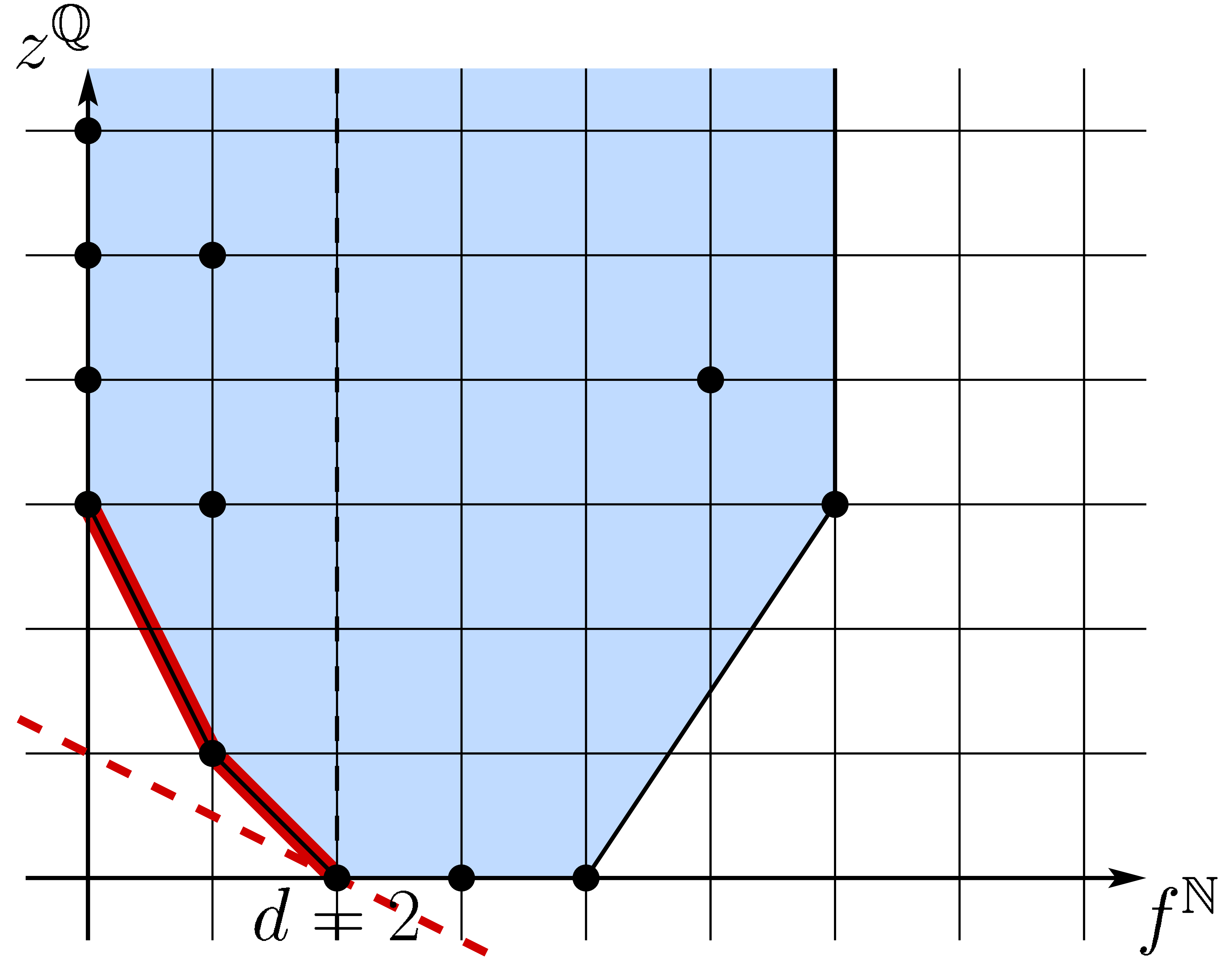
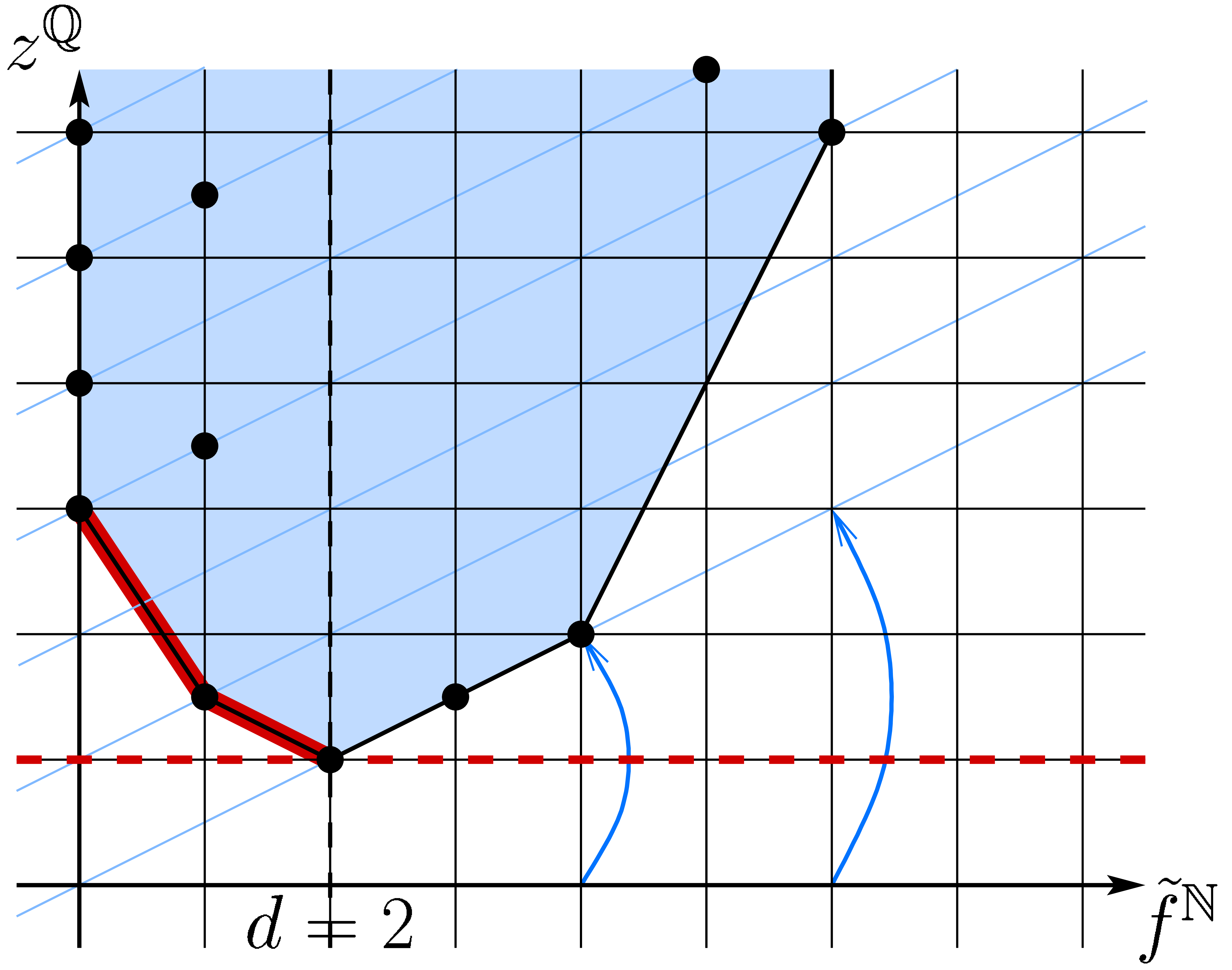
 .
. and the edges
of the Newton polygon with slope
and the edges
of the Newton polygon with slope  have
been highlighted. Notice that the Newton degree
have
been highlighted. Notice that the Newton degree  corresponds to the first coordinate of the rightmost point on an
edge with slope
corresponds to the first coordinate of the rightmost point on an
edge with slope  on the Newton polygon.
 ).
).
 ,
,

 .
. ,
, in the case of heavy transbases and
 otherwise.
 ,
, ,
, (i.e. the coefficient of
  in the
lexicographical series
in the
lexicographical series  (by
convention,
(by
convention,  if
if  ),
), .
. ,
, is again a transbasis
of the same kind as
is again a transbasis
of the same kind as  can be expanded w.r.t.
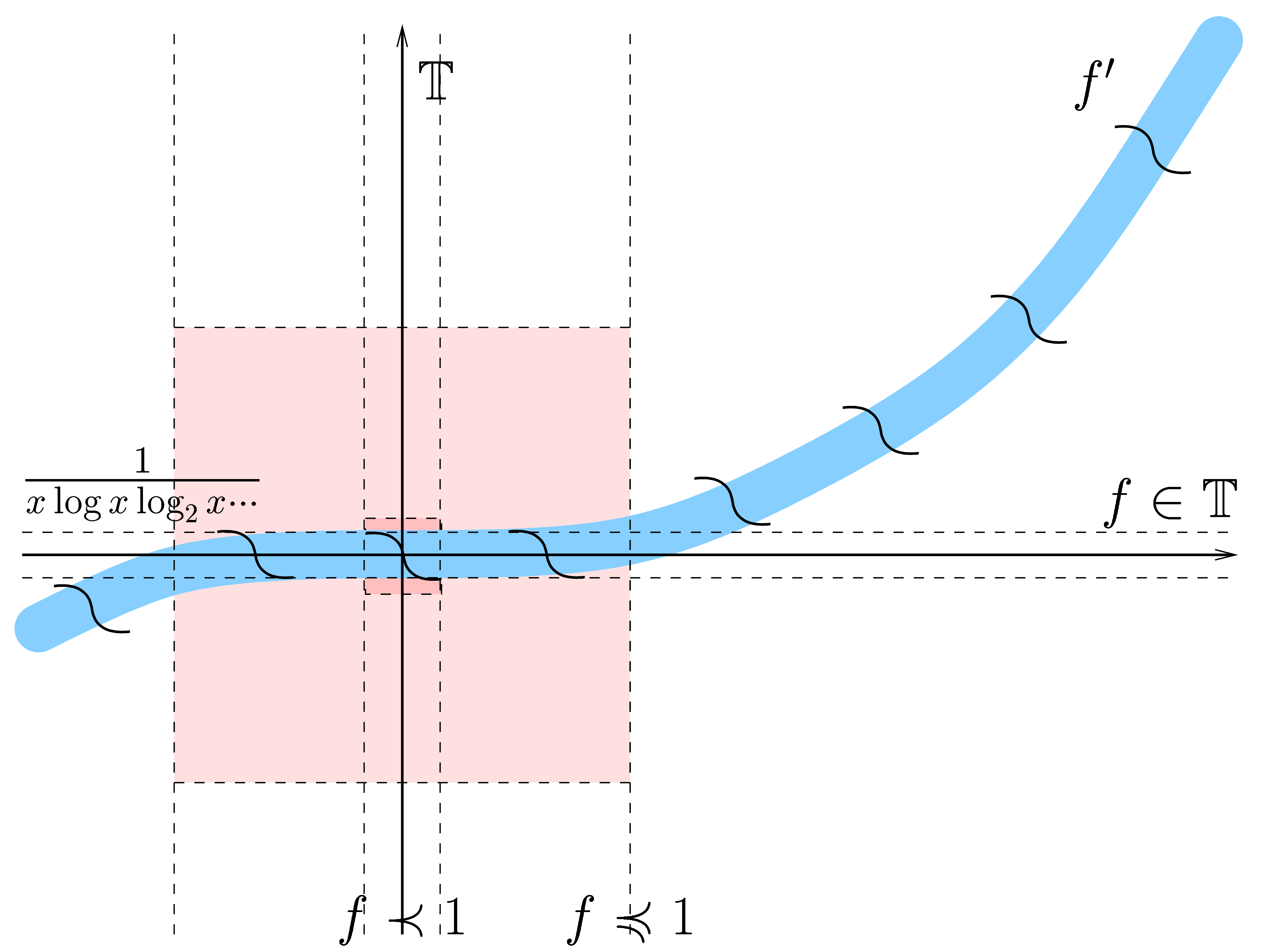
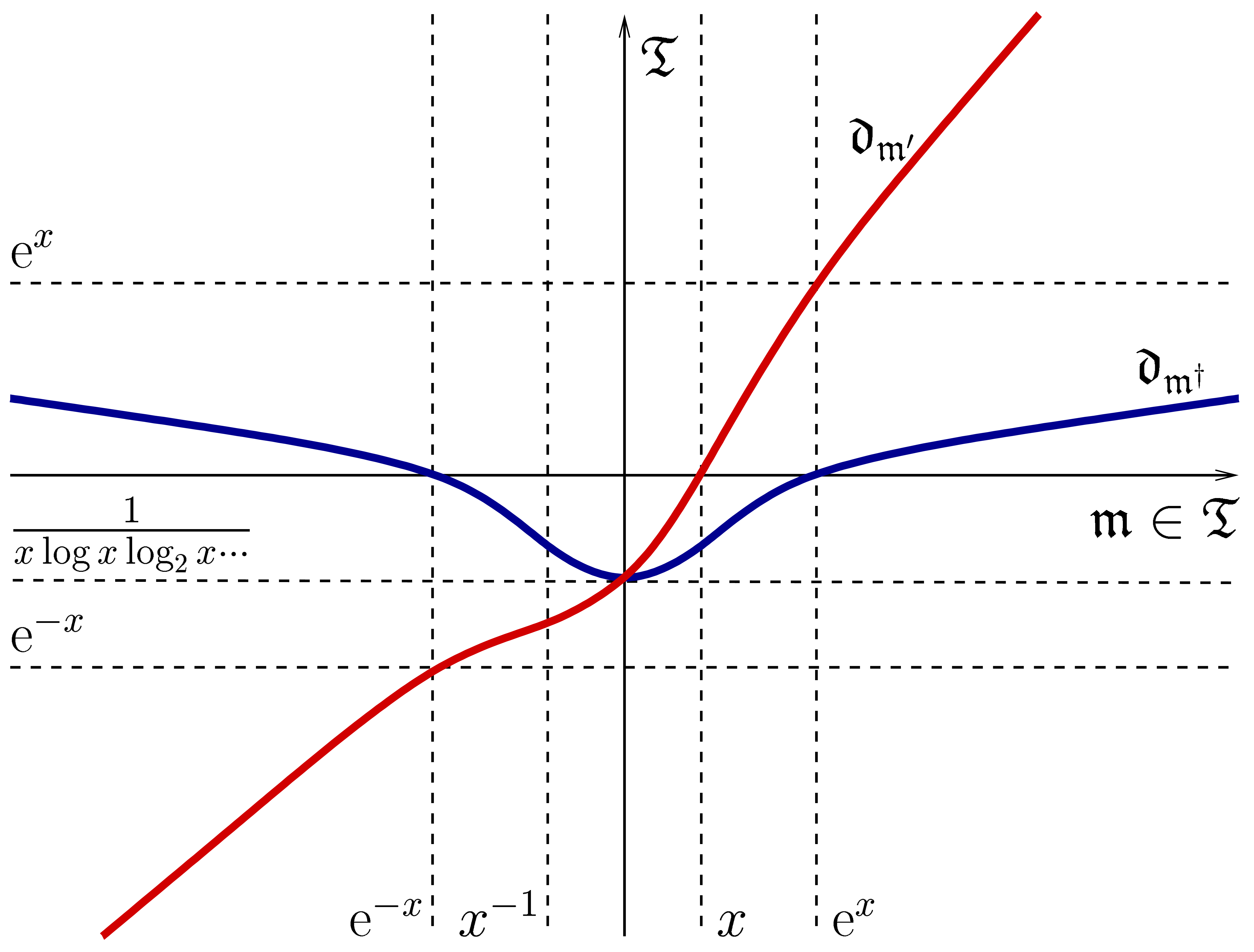
 and
and  for transmonomials (using
logarithmic coordinates).
for transmonomials (using
logarithmic coordinates).
 with
with  .
. .
. into
into  ,
, and
and  ,
,
 so that (
 .
. .
. and
and
 .
. and
and  for
all
for
all  .
. ,
, is not strongly summable, as it should be. Hence
  ,
, .
. is divergent. Deduce that
  ,
, .
. be such that
  and
and 
 be infinitesimal linear grid-based operators
(i.e.
be infinitesimal linear grid-based operators
(i.e.  for
for  ).
).


 whenever
  .
. whenever
  for
all
for
all  if for all
  with
with  .
. .
.


 ,
,
 ,
, .
. be two flat subspaces of
  .
. .
.


 ,
, .
. .
. for all
  .
. ,
, for all
  .
. .
. and
and

 ,
, .
.


 and
and  ,
, .
. .
. term is divided by


 ,
, and let
  be such that


 and
and 
 and the interval
 .
. quasi-ordering
 equivalent elements w.r.t.
quasi-ordering
equivalent elements w.r.t.
quasi-ordering
 set of non-empty words over
  ordering defined by
  final segment generated by
  initial segment generated by
  subset of non-zero elements in
  subset of negative or zero elements in
 subset of strictly negative elements
in
subset of strictly negative elements
in  absolute value of
 and
and 


 monomials
 ring of grid-based series in
  coefficient of
  natural multivariate series in
  recursive multivariate series in
  series with
  purely infinite part of
  constant part of
  infinitesimal part of
  set of purely infinite elements in

 set of infinitesimal elements in
  set of bounded elements in
  the series
 restriction of
  collection of families with values in
 Cartesian product of families
  application of a function
 collection of strongly summable
families over
collection of strongly summable
families over  family of monomials occurring in
  composition of
 series in
  subset of convergent grid-based series
in
subset of convergent grid-based series
in 
 field of grid-based transseries in
 transseries of exp. height
  and log. depth
 field of exponential transseries
 of
of  of
of  contraction
  of
of
 dilatation
  of
of
 field of convergent transseries
 distinguished integral of
  right composition with
  scalar product
  of
of  composition of multilinear grid-based
operators
composition of multilinear grid-based
operators
 operator support of
  sets of operators
  on
on 
 and
and  set of strongly multilinear
 set of grid-based operators from
 atomic
  arity of an atomic operator
  inputs of an atomic operator
  output of an atomic operator
 composition of atomic families
  alternative notation for dominant
coefficient
alternative notation for dominant
coefficient 
 upward and downward shiftings of
  Stirling numbers of the first kind
 Stirling numbers of the second kind

 and
and 
 space of operators of the form
 algebraic part of
  derivative of differential operator
 complexification
  of
of  spectral part of

 coefficient of
  shorthand for
 (total) degree of
  shorthand for
 (normalized) coefficient of
 weight of
  weighted differential valuation of


 shorthand for
 coefficient of
  upward and downward shiftings of
  Newton degree of
 -equalizer
 maximal open interval containing
  the interval
 the interval
 minimal element of
  maximal element of
 shorthand for

 set
set  of finite
cuts in
of finite
cuts in  width of
  serial completion of
 shorthand for

 integral coordinates of
  sign of
  sign of
  sign of
  sign of