Static bounds for straight-line programs Joris van der Hoevena, Grégoire Lecerfb, Arnaud Minondoc Laboratoire d'informatique de l'École polytechnique (LIX, UMR 7161 CNRS) CNRS, École polytechnique, Institut Polytechnique de Paris Bâtiment Alan Turing, CS35003 1, rue Honoré d'Estienne d'Orves 91120 Palaiseau, France a. Email: vdhoeven@lix.polytechnique.fr b. Email: lecerf@lix.polytechnique.fr c. Email: minondo@lix.polytechnique.fr Preliminary version of June 10, 2025

. Grégoire Lecerf and Arnaud Minondo have been supported by the French ANR-22-CE48-0016 NODE project. Joris van der Hoeven has been supported by an ERC-2023-ADG grant for the ODELIX project (number 101142171).

Funded by the European Union. Views and opinions expressed are however those of the author(s) only and do not necessarily reflect those of the European Union or the European Research Council Executive Agency. Neither the European Union nor the granting authority can be held responsible for them.

1.Introduction

Interval arithmetic is a popular technique to calculate guaranteed error bounds for approximate results of numerical computations [2, 13, 16–21]. The idea is to systematically replace floating point approximations by small intervals around the exact numbers that we are interested in. Basic arithmetic operations on floating point numbers are replaced accordingly with the corresponding operations on intervals. When computing with complex numbers or when working with multiple precision, it is more convenient to use balls instead of intervals. In this paper, we will always do so and this variant of interval arithmetic is called ball arithmetic [8, 14].

Unfortunately, ball arithmetic suffers from a non-trivial overhead: floating point balls take twice the space of floating point numbers and basic arithmetic operations are between two and approximately ten times more expensive. For certain applications, it may therefore be preferable to avoid the systematic use of balls for individual operations. Instead, one may analyze the error for larger groups of operations. For instance, when naively multiplying two double precision matrices whose coefficients are all bounded by in norm (say), then it is guaranteed that the maximum error of an entry of the result is bounded by , without having to do any individual operations on balls.

The goal of this paper is to compute reliable error bounds in a systematic fashion, while avoiding the overhead of ball arithmetic. We will focus on the case when the function that we wish to evaluate is given by a straight-line program (SLP). Such a program is essentially a sequence of basic arithmetic instructions like additions, subtractions, multiplications, and possibly divisions [5]. For instance, matrix multiplication can be computed using an SLP. The SLP framework is actually surprisingly general: at least conceptually, the trace of the execution of a more general program that involves loops or subroutines can often be regarded as an SLP [11, section 3].

So consider a function that can be computed using an SLP, where or . Given and , let denote the ball with center and radius . We will consider several problems:

Q1

Given an approximate evaluation using floating point arithmetic, can we efficiently compute a bound for the error?

Q2

Given and , can we efficiently compute such that ?

Q3

Given balls , an index , and , can we efficiently compute a bound for on ?

Here “efficiently” means that the cost of the bound computation should not exceed , ideally speaking. In particular, the cost should not depend on the length of the SLP, but we do allow ourselves to perform precomputations with such a higher cost. We may regard Q1 as a special case of Q2 by taking . If , then Q3 becomes essentially a special case of Q2, since we may use as the required bound.

Of course, there is a trade-off between the cost of bound computations and the sharpness of the obtained bounds. We will allow our bounds to be less sharp than those obtained using traditional ball arithmetic. But we still wish them to be as tight as possible under the constraint that the cost of the bound computations should remain small.

We start with the special case when the centers lie in some fixed balls . For this purpose we introduce a special variant of ball arithmetic, called matryoshka arithmetic: see section 2. A matryoshka is a ball whose center is itself a ball and its radius is a number in . Intuitively speaking, a matryoshka allows us to compute enclosures for “balls inside balls”. By evaluating at matryoshki with centers and zero radii, we will be able to answer question Q1: see section 3. Using this to compute bounds for the gradient of on , we will also be able to answer question Q2 in the case when .

In section 3, we will actually describe a particularly efficient way to evaluate SLPs at matryoshki. For this, we will adapt transient ball arithmetic from [10]. This variant of ball arithmetic has the advantage that, during the computations of error bounds for individual operations, no adjustments are necessary to take rounding errors into account. We originally developed this technique for SLPs that only use ring operations. In section 4, we will extend it to SLPs that may also involve divisions.

For polynomial SLPs that do not involve any divisions, we will show in section 5 that it is actually possible to release the condition that must be contained in fixed balls . The idea is to first reduce to the case when the components with are homogeneous. Then for some , so we may always rescale such that it fits into the unit poly-ball . We may then apply the theory from sections 2 and 3. Reliable numeric homotopy continuation [4, 6, 7, 9, 15] is a typical application for which it is important to efficiently evaluate polynomial SLPs at arbitrary balls.

Our final section 6 is devoted to question Q3. The main idea is to compute bounds for the on balls with the same centers but larger radii. We will then use Cauchy's formula to obtain bounds for the derivatives of without having to explicitly compute these derivatives. Bounds for the derivatives of are in particular useful when developing reliable counterparts of Runge–Kutta methods for the integration of systems of ordinary differential equations. We intend to provide more details about this application in an upcoming paper.

2.Different types of ball arithmetic

2.1.IEEE floating point arithmetic and notation

Throughout this paper, we assume that we work with a fixed floating point format that conforms to the IEEE 754 standard. We write for the bit precision, i.e. the number of fractional bits of the mantissa plus one. We also denote the minimal and maximal allowed exponents by and . For IEEE 754 double precision numbers, this means that , and . We denote the set of hardware floating point numbers by . Given an -algebra , we will also denote the corresponding approximate version by . For instance, if , then we have .

The IEEE 754 standard imposes correct rounding of all basic arithmetic operations. In this paper we will systematically use the rounding to nearest mode. We denote by the result of rounding according to this mode. The quantity stands for the corresponding rounding error, which may be . Given a single operation , it will be convenient to write for . For compound expressions , we will also write for the full evaluation of using the rounding mode . For instance, .

We denote by any upper bound function for that is easy to compute. In absence of underflow, one may take . If we want to allow for underflows during computations, then we can take instead, where is the smallest positive subnormal number in . If , then we may still take since no underflow occurs in that special case. See [10, section 2.1] for more details about these facts.

For bounds on rounding errors, the following lemma will be useful.

Proof. Let for all . Since , we have

2.2.Ball arithmetic

Let be an -algebra and let be a norm on . We will typically take or , but more general normed algebras are also allowed. Given and , let be the closed ball with center and radius . We denote by the set of all such balls.

The aim of ball arithmetic is to provide a systematic way to bound the errors of numerical computations. The idea is to systematically replace numerical approximations of elements in by balls that are guaranteed to contain the true mathematical values. It will be useful to introduce a separate notation for this type of semantics: given a ball and a number, we say that encloses if , i.e.

We also introduce poly-balls, which are vectors of balls, for situations where it is required to reason “coordinate wise”. For all and all , we denote the poly-ball . We extend this enclosure relation to poly-balls and as follows:

(2.1)

In the sequel, we will use a bold font for ball enclosures and a normal font for values at actual points. Note that the smallest enclosure of is the “exact” ball , and we will regard as being embedded into in this way.

Let us now recall how to perform arithmetic operations in a way that is compatible with the “enclosure semantics”. Given a function , a ball lift of is a function that satisfies the inclusion property

for all and . (Note that we voluntarily used the same name for the function and its lift.) For instance, the basic arithmetic operations admit the following ball lifts:

			(2.2)
			(2.3)

Other operations can be lifted in a similar way (in section 4 below, we will in particular study division). We can also extend the norm from to via

			(2.4)

The extended norm is sub-additive, sub-multiplicative, and positive definite.

2.3.Matryoshka arithmetic

For any ball , we have , so is clearly not an additive group in the mathematical sense. Nonetheless, we may consider to be a normed -algebra from a computer science perspective, because all the relevant operations , and are “implemented”. Allowing ourselves this shortcut, we may apply the theory from the previous subsection and formally obtain a ball arithmetic on . It turns out that this construction actually makes sense from a mathematical perspective, provided that we appropriately adapt the semantics for the notion of “enclosure”.

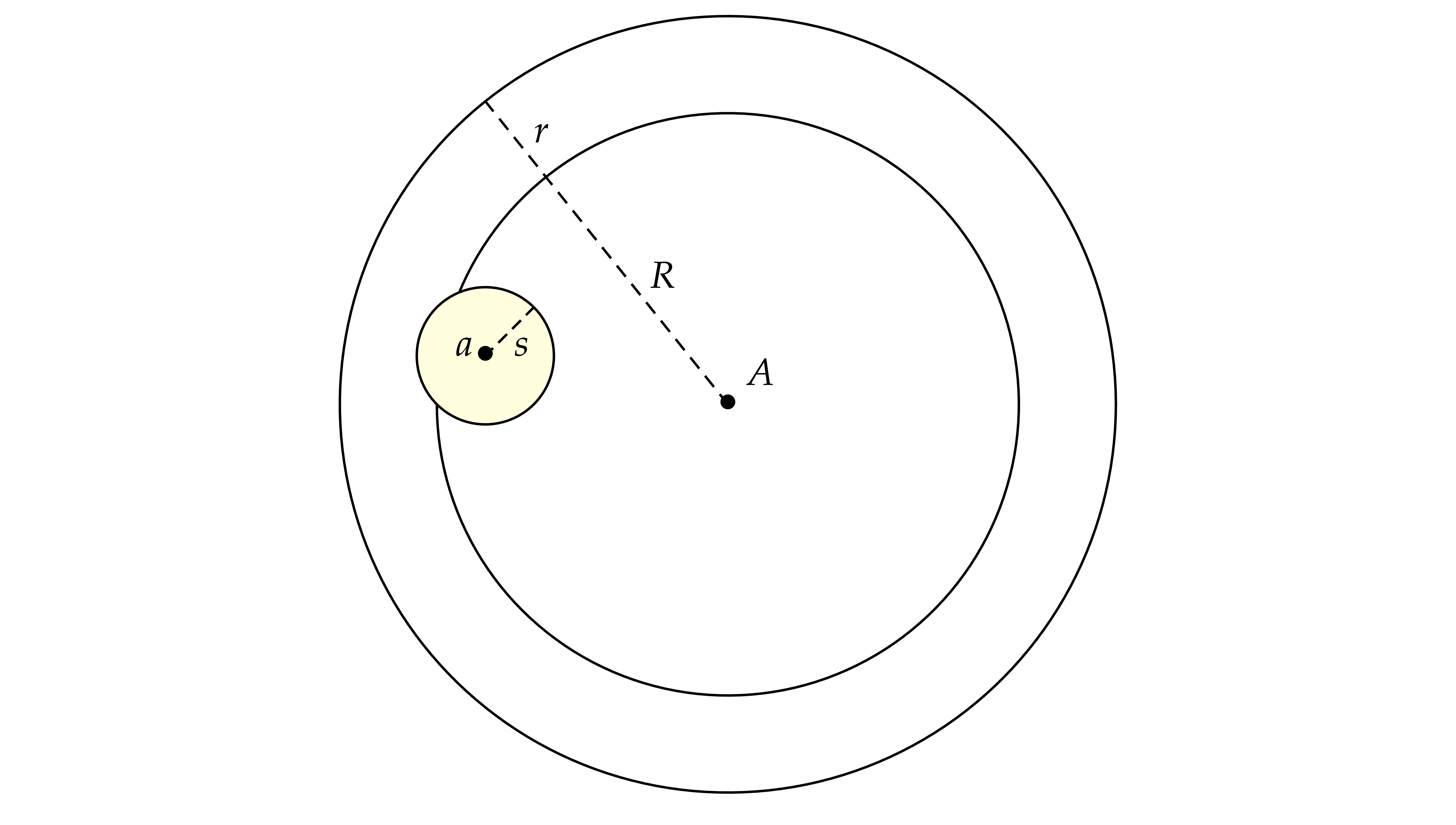
Let . An element of will be called a matryoshka. Given a matryoshka , we call its center, its large radius, and its small radius. The appropriate enclosure relation for matryoshki is defined as follows: given a matryoshka and a ball , we define

Conceptually, the “small embedded ball” is contained in the matryoshka, which corresponds to the “big ball” : see Figure 2.1 . The enclosure relation naturally extends to vectors as in ( 2.1 ).

Figure 2.1. Representation of an embedded ball inside a matryoshka.

We use the abbreviation for the set of matryoshki. A function is said to lift to if it satisfies the inclusion principle:

for all and . Exactly the same formulas (2.2) and (2.3) can be used in order to lift the basic arithmetic operations:

for all . (Note that it was this time convenient to use , as a notation for the centers of our matryoshki.) We may also extend the norm on to matryoshki via

which again remains sub-additive, sub-multiplicative, and positive definite.

Remark 2.2. In principle, we could repeat the process and recursively consider matryoshki as centers of even larger matryoshki. While attractive from a folkloric perspective, it turns out that the basic matryoshki are more efficient for the applications we know of.

2.4.Rounded and transient ball arithmetic

We will write and for the approximate versions of and when working with machine floating point numbers in instead of exact real numbers in . In that case, the formulas from section 2.2 and 2.3 need to be adjusted in order to take into account rounding errors. For instance, if , then one may replace the formulas (2.2), (2.3), and (2.4) by

(2.5)

See, e.g., [10]. We will call this rounded ball arithmetic.

Unfortunately, these formulas are far more complicated than (2.2), (2.3), and (2.4), so bounding the rounding errors in this way gives rise to a significant additional computational overhead. An alternative approach is to continue to use the non-adjusted formulas

(2.6)

This type of arithmetic was called transient ball arithmetic in [10]. This arithmetic is not a ball lift, but we will see below how to take advantage of it by inflating the radii of the input balls of a given SLP.

Of course, we need to carefully examine the amount of inflation that is required to ensure the correctness of our final bounds. This will be the purpose of the next section in the case where we evaluate an entire SLP using transient ball arithmetic. We denote by a quantity that satisfies and

(2.7)

for all and , in absence of underflows and overflows. One may for instance take and , whenever ; see [10, Appendix A of the preprint version].

We recall the following lemma, which provides a useful error estimate for the radius of a transient ball product.

Lemma 2.3. [10, Lemma 3] For all and such that the computation of

involves no underflows or overflows, we have .

In the presence of overflows or underflows, additional adjustments are required. Overflows actually cause no problems, because the IEEE 754 standard rounds every number beyond the largest representable floating point number to infinity, so the radii of balls automatically become infinite whenever an overflow occurs. In order to protect ourselves against underflows, the requirements (2.7) need to be changed into

(2.8)

Here we recall that additions and subtractions never lead to underflows. If , then we may take . If , then a safe choice is (in fact, is sufficient for multiplication). We refer to [10, section 3.3] for details.

2.5.Transient matryoshka arithmetic

Taking instead of for our center space, the formulas (2.6) naturally give rise to transient matryoshka arithmetic:

Here we understand the operations , , and on the centers are done use transient ball arithmetic.

We will need an analogue of Lemma 2.3 for matryoshki. Given balls and in , we define . In what follows, let be such that and

(2.9)

for all and , in absence of underflows and overflows.

Let . Given and , Lemma 2.3 gives ; similarly we have

This implies

It thus suffices to take for (2.9) to hold in the case of multiplication. Simpler similar computations show that this is also sufficient for the other operations. We can now state the analogue of Lemma 2.3.

Lemma 2.4. For all and such that the computation of

involves no underflows or overflows, we have .

Proof. The same as the proof of [10, Lemma 1], mutatis mutandis.

3.Evaluating straight line programs

3.1.Straight-line programs

A straight-line program over a ring is a sequence of instructions of the form

where are variables in a finite ordered set , constants in , and . Variables that appear for the first time in the sequence in the right-hand side of an instruction are called input variables. A distinguished subset of the set of all variables occurring at the left-hand side of instructions is called the set of output variables. Variables which are not used for input or output are called temporary variables and determine the amount of auxiliary memory needed to evaluate the program. The length of the sequence is called the length of .

Let be the input variables of and the output variables, listed in increasing order. Then we associate an evaluation function to as follows: given , we assign to for , then evaluate the instructions of in sequence, and finally read off the values of , which determine .

To each instruction , one may associate the remaining path lengths as follows. Let , and assume that have been defined for some . Then we take , where are those indices such that is of the form with , , and . If no such indices exist, then we set . Similarly, for each input variable we define , where are those indices such that is of the form with , , and . We also define , where are the input variables of and all indices such that is of the form .

Example 3.1. Let us consider , of length . The input variables are and , and we distinguish as the sole output variable. This SLP thus computes the function . The associated computation graph, together with remaining path lengths are as pictured:

3.2.Transient ball evaluations

Our goal is to evaluate SLPs using transient ball arithmetic from section 2.4 instead of rounded ball arithmetic. Transient arithmetic is faster, but some adjustments are required in order to guarantee the correctness of the end-results. In order to describe and analyze the correctness of these adjustments, it is useful to introduce one more variant of ball arithmetic.

In semi-exact ball arithmetic, the operations on centers are approximate, but correctly rounded, whereas operations on radii are exact and certified:

where and . The extra terms in the radius ensure that these definitions satisfy the inclusion principle.

In order to measure how far transient arithmetic can deviate from this idealized semi-exact arithmetic, let be the -th harmonic number and let for all . The following theorem shows how to certify transient ball evaluations:

Theorem 3.2. [10, Theorem 5] Let be an SLP of length as above and let be an arbitrary parameter such that , where is as in (2.7). Consider two evaluations of for different types of ball arithmetic. For the first evaluation, we use semi-exact ball arithmetic with . For the second evaluation, we use transient ball arithmetic with the additional property that any input or constant ball is replaced by a larger ball with

where

Assume that no underflow or overflow occurs during the second evaluation. For any corresponding outputs and for the first and second evaluations, we then have .

Given a fixed and , we note that we may take and such that . The value of the parameter may be optimized as a function of the SLP and the input. Without entering details, should be taken large when the input radii are small, and small when these radii are large. The latter case occurs typically within subdivision algorithms. For our main application when we want to compute error bounds, the input radii are typically small or even zero.

For our implementations in Mathemagix [12] and JIL [1], we found it useful to further simplify the bounds from Theorem 3.2, assuming that is “sufficiently small”.

Corollary 3.3. With the notation from Theorem 3.2, assume that . In order to apply Theorem 3.2, it is sufficient to take and

Proof. The harmonic series satisfies the well-known inequality , of which we only use the right-hand part. Lemma 2.1 also yields . Given that , it follows that

Therefore,

3.3.From balls to matryoshki

The semi-exact ball arithmetic from the previous subsection naturally adapts to matryoshki as follows: given and , we define

where is extended to balls via

Recall that denotes an upper bound on the rounding errors involved in the computation of the norm of . Operations on centers use the semi-exact arithmetic from the previous subsection. This arithmetic is therefore a matryoshka lift of the elementary operations. The following theorem specifies the amount of inflation that is required in order to certify SLP evaluations using “transient matryoshka arithmetic”.

Theorem 3.4. Let , and let be as in Theorem 3.2. Consider two evaluations of for two different types of arithmetic. For the first evaluation, we use semi-exact matryoshka arithmetic with . For the second evaluation, we use transient matryoshka arithmetic with the additional property that any input or constant ball is replaced by a larger ball with

Assume that no underflow or overflow occurs during the second evaluation. For any corresponding outputs and for the first and second evaluations, we then have and .

Proof. The theorem essentially follows by applying Theorem 3.2 twice: once for the big and once for the small radii. This is clear for the big radii and since the formulas for the big radii of matryoshki correspond with the formula for the radii of the corresponding ball arithmetic. For the small radii, we use essentially the same proof as in [10]. For convenience of the reader, we reproduce it here with the required minor adaptations.

Let be the value of the variable after the evaluation of using transient matryoshki arithmetic. It will be convenient to systematically use star superscripts for the corresponding value when using semi-exact matryoshka arithmetic. Let us show by induction on that:

(3.1)

If is of the form , then we are done since . Otherwise, is of the form . Writing , we claim that

This holds by assumption if is an input variable. Otherwise, let be the largest index such that . Then by construction of , whence our claim follows from the induction hypothesis. Similarly, writing , we have .

Having shown our claim, let us first consider the case where . In this case we obtain

Combined with (2.9) and the inequalities

(3.2)

we deduce:

In case when , we obtain

Combined with Lemma 2.4, the inequalities (3.2), (2.9), and successively imply

which achieves the induction. Then, for all , we define

so that . By the inequality that we imposed on , we have . Using a second induction over , let us next prove that

(3.3)

Assume that this inequality holds up until order . If is of the form then we are done by the fact that . If is of the form , then let be the largest integers so that and , so we have ,

and

using (3.1). In particular, we obtain . We denote by (resp. ) the matryoshka corresponding to the value of (resp. ) in the semi-exact evaluation. Their corresponding values for the transient evaluation are denoted without the star superscript. Thanks to Theorem 3.2, we know that , whence since . With and as above, using (3.3) and (2.9), it follows that

If is of the form , then, thanks to Lemmas 2.3, 2.4, and inequality (3.3) a similar calculation yields

which completes the second induction and the proof of this theorem.

Remark 3.5. In [10, section III.C], it is discussed how to manage underflows and overflows in Theorem 3.2. A similar discussion applies to Theorem 3.4.

3.4.Applications

Let us now give two direct applications of matryoshka arithmetic. Assume that we are given an SLP that computes a function and denote by the function obtained by evaluating using approximate floating point arithmetic over . Matryoshki yield an efficient way to statically bound the error for inside some fixed poly-ball, as follows:

Proposition 3.6. Let be a fixed poly-ball and . Let be a poly-matryoshka lift of and . Then for all with and , we have

Proof. Let be a ball lift for which satisfies the matryoshka lift property. Since by assumption, we have

for some . The ball lift property also yields

so for .

As our second application, we wish to construct a ball lift of that is almost as efficient to compute as itself, provided that the input balls are included into fixed large balls as above. For this, we first compute bounds for the Jacobian matrix of :

(3.4)

For this, it suffices to evaluate a ball lift of the Jacobian of at , which yields a matrix , after which we take . We recall that an SLP for the computation of the Jacobian can be constructed using the algorithm by Baur and Strassen [3].

Proposition 3.7. Let for all integers and . With the above notation, assume that , and let be as in Proposition 3.6. For every with , let

Then is a ball lift of . (Note that this lift is only defined on the set of such that .)

Proof. Let . Then, for , we have

by (3.4) and the mean value theorem. In other words,

Applying Proposition 3.6, it follows that

By computing the sum via a balanced binary tree and using (2.8), we obtain

where we also used Lemma 2.1 and the fact that the computation of is exact.

4.Division

It is classical to extend ball arithmetic to other operations like division, exponentiation, logarithm, trigonometric functions, etc. In this section, we will focus on the particular case of division. It will actually suffice to study reciprocals , since .

Divisions and reciprocals raise the new difficulty of divisions by zero. We recall that the IEEE 754 provides a special not-a-number element NaN in that corresponds to undefined results. All arithmetic operations on NaN return NaN, so we may check whether some error occurred during a computation, simply by checking whether one of the return values is NaN. For exact arithmetic, we will assume that is extended in a similar way with an element such that .

4.1.Reciprocals of balls

In the remainder of this section, assume that or . In order to extend reciprocals to balls, it is convenient to introduce the function

Then the exact reciprocal of a ball can be defined as follows:

(4.1)

where we note that

If then we may also use the following formula

(4.2)

for transient ball arithmetic and

(4.3)

for semi-exact ball arithmetic.

We assume that the rounded counterpart of the reciprocal verifies the condition

(4.4)

for all invertible in . For IEEE 754 arithmetic, this condition is naturally satisfied for when , and in absence of overflows and underflows. If and , then we compute reciprocals using the formula

For this definition, we have

Now

whence

For , it follows that

Consequently,

This shows that we may take .

Let us denote and assume that . We are now in a position to prove a counterpart of Lemma 2.3 for division.

Lemma 4.1. Let and be such that . Assume that the computation of

involves no overflows and no underflows. Then .

Proof. We have

whence

whence

We conclude by observing that , since .

4.2.Transient evaluation

We adapt the definition of the remaining path length to our extended notion of SLPs with reciprocals. We now take , where are those indices such that is of the form with , , and , or is of the form and . Lemma 4.1 allows us to extend Theorem 3.2 as follows.

Theorem 4.2. With the setup from Theorem 3.2, assume that and that may also contain reciprocals. During the second evaluation, assume that no underflow or overflow occurs and that for every computation of a reciprocal of , where . Assume in addition that and that the following two inequalities hold:

Then for any corresponding outputs and for the two evaluations.

Proof. We adapt the proof of [10, Theorem 5], by showing that the two inductions still go through in the case of reciprocals. For the first induction, consider an instruction , where and . Recall that

Using , , and Lemma 2.1, we note that

			(4.5)

Combined with Lemmas 4.1 and 2.1, we deduce that

For the second induction, we redefine

Assume , let (resp. ) be the value of in the semi-exact evaluation (resp. transient evaluation), and let be the biggest index so that . Then

The two inductions still hold for the other operations since we increased and .

If the conditions of the theorem are all satisfied for a given input poly-ball , then we note that the numeric evaluation of the SLP at any point with never results in a division by zero. Conversely however, even when all these numerical evaluations are legit, it may happen that the condition that is violated for the computation of some reciprocal . This can either be due to an overly optimistic choice of or to the classical phenomenon of overestimation.

Intuitively speaking, a low choice of means that balls that need to be inverted should neatly steer away from zero, even when inflating the radius by a small constant factor. In fact, this is often a reasonable requirement, in which case one may simply take . A somewhat larger choice like remains appropriate and has the advantage of increasing the resilience of reciprocal computations (the condition being easier to satisfy). Large values of deteriorate the quality of the obtained bounds for a dubious further gain in resilience.

4.3.Reciprocals of matryoshki

The formulas (4.1), (4.2), and (4.3) for reciprocals can again be specialized to matryoshki modulo the precaution that we should interpret as a lower bound for the norm. For and , this leads to the definitions

where we use the lower bound notation . In addition to (2.9), we will assume that the rounded counterpart of the reciprocals also verifies the condition

(4.6)

for all invertible balls in . For what follows, let .

Lemma 4.3. Let be such that . Let be such that and . If the computation of

involves no overflows and no underflows, then .

Proof. From

and

we obtain

It follows that

Using and , we have

and then

We are now ready to extend Theorem 3.4 to SLPs with reciprocals.

Theorem 4.4. Let be such that and let . With the setup from Theorem 3.4, assume that and that may also contain reciprocals. During the second evaluation, assume that no underflow or overflow occurs and that and hold for every computation of a reciprocal of . Assume in addition that and that the following two inequalities hold:

Then and for any corresponding outputs and for the first and second evaluations.

Proof. We adapt the proof of Theorem 3.4 by showing that the two inductions still go through in the case of reciprocals. For the first induction, consider an instruction , where , with and . Recall that

Using Lemma 4.3, the identity , as well as (4.5) and (3.2), we obtain

For the second induction, we redefine

Assume , let (resp. ) be the value of in the semi-exact evaluation (resp. transient evaluation), and let be the biggest index so that . Then Lemma 4.3 implies

The two inductions still hold for the other operations since we increased and .

Similar comments as those made after Theorem 4.2 also apply to the above theorem. In particular, we recommend taking .

5.Global projective bounds

In the previous sections we have focussed on more efficient algorithms for the reliable evaluation of functions on fixed bounded poly-balls. This technique applies to very general SLPs that may involve operations like division, which are only locally defined. Nonetheless, polynomial SLPs, which only involve the ring operations are important for many applications such as numerical homotopy continuation. In this special case, we will show how remove the locality restriction and allow for the global evaluation of such SLPs in a reliable and efficient way.

5.1.Homogenization of SLPs

Consider a polynomial map

for polynomials . Given , the polynomial is not homogeneous, in general, but there exists a homogeneous polynomial such that . This polynomial is unique up to multiplication by powers of . The polynomials give rise to a polynomial map

which we call a homogenization of .

Assume now that the map can be computed using an SLP of length without divisions. Let us show how to construct an SLP such that is a homogenization of . Consider the formal evaluation of over , by applying to the input arguments . Then the output value and the input arguments and of an instruction of the form () are polynomials in that we denote by , and , respectively (for instructions , we set ). We can recursively compute upper bounds , , (abbreviated as , , ) for the total degrees of these polynomials:

• If is of the form , then we take .

• If is of the form , then .

• If is of the form , then .

Here (resp. ) whenever (resp. ) is an input variable.

Now consider the program obtained by rewriting each instruction as follows:

• If is of the form or , then is rewritten into itself.

• If is of the form with , then is rewritten into itself.

• If is of the form with , then is rewritten into two instructions and , for some new auxiliary variable .

• If is of the form with , then is rewritten into two instructions and , for some new auxiliary variable .

By induction, one verifies that the image of under this rewriting computes the unique homogenization of of degree for . We obtain by prepending with instructions that compute all powers that occur in . This can for instance be done using binary powering: and for all .

Example 5.1. Applying the homogenization procedure to the left-hand SLP below, we obtain the right-hand one:

In this example, , , and . In the last instruction, we thus have , whence the exponent in .

Remark 5.2. In the worst case, computing the powers of using binary powering may give rise to a logarithmic overhead. For instance, there is a straightforward SLP of length proportional to that computes the polynomials for . But when computing using binary powering in order to compute its homogenization, the length of is proportional to .

An alternative way to compute the required powers is to systematically compute and for all . In that case and can always be obtained using a simple multiplication and the length of remains bounded by for an SLP of length . Of course, this requires division to be part of the SLP signature, or to be passed an argument, in addition to .

Consider an output variable with and denote by and the -th component of and , respectively. If is largest with , then we define , and we note that is the unique homogenization of of degree . Let and define for any . For any and , it then follows that

(5.1)

We will denote by the polynomials with for all .

5.2.Global bounds through homogenization

With the notation from the previous subsection, assume that with or . Suppose that we wish to evaluate at a point and let

(5.2)

Of course, we may simply evaluate at , which yields . But thanks to (5.1), we also have the projective evaluation method

The advantage here is that

(5.3)

so we only evaluate at points in the poly-ball . This allows us to apply the material from the previous sections concerning the evaluations of SLPs at points inside a fixed ball. Note that we may easily add the function to SLPs since its computation is always exact. If then we apply to the real and imaginary parts.

For instance, let be the evaluation of at using ball arithmetic and set for . Then we have

(5.4)

for all and . Consequently, we may compute upper bounds for in time , which is typically much smaller than the length of .

We may use such global bounds for the construction of more efficient ball lifts, although the resulting error bounds may be less sharp. For this, we first evaluate the Jacobian matrix of at , which yields bounds

(5.5)

for all , , and . For any ball with for , we then have

(5.6)

This allows us to compute an enclosure of using a single evaluation of at plus extra operations (the quantity can be further reduced to by replacing the by or ).

Similarly, if is any ball, then we define

(5.7)

For , the relations (5.1) and (5.6) now yield

(5.8)

(If , then is a constant, and we may use zero as the radius.) This allows us to compute an enclosure of using one evaluation of at plus extra operations in . Note that the homogenization was only required in order to compute the constants , but not for evaluating the right-hand side of (5.8) at a specific .

5.3.Managing rounding errors

In the previous subsection, we assumed infinitely precise arithmetic over or . Let us now show how to adapt this material to the case when , where or . As usual, assume , and let us first show how to deal with rounding errors in the absence of overflows and underflows. We first replace (5.2) by

and verify that

We have

Let . Evaluating at , for the matryoshka , by Proposition 3.6 for instance, we may compute a with

for all , as well as

for all with . It follows that

Setting

we then get

			(5.9)

Note that for all and we have

whence . Consequently, provided that , the bound (5.9) simplifies into

(5.10)

This yields an easy way to compute error bound

(5.11)

for the approximate numeric evaluation of at any point .

Let us now turn to the bound (5.4). Using traditional ball arithmetic (formulas (2.5)) over , we may still compute with for all with . Then we simply have

for all , since . In a similar way, bounds that satisfy (5.5) can be computed using traditional ball arithmetic. For any ball and with we notation from (5.7), the enclosure (5.8) still holds. Combining

with (5.10), this yields

Hence

where

(5.12)

This yields a ball lift for that is almost as efficient to compute as a mere numeric evaluation of .

Let us finally analyze how to deal with underflows and overflows. Let be such that (2.8) holds. As long as the computation of does not underflow, the inequality remains valid, even in the case of overflows (provided that ). Consequently, the relation (5.10) still holds, so it suffices to replace (5.11) by

This indeed counters the possible underflow for the multiplication of with . Note that the relation trivially holds in the case when the right-hand side overflows, which happens in particular when the computation of overflows. Similarly, it suffices to replace (5.12) by

If the computation of does not overflow, but the computation of underflows, then the IEEE 754 norm implies that we must have , where is the largest positive floating point number in with . Consequently, the computation overflows whenever , provided that we compute this product as times . The adjusted bounds are therefore valid in general.

6.Bounding derivatives

For several applications, it is useful to not only compute bounds for the function itself, but also for some of its iterated derivatives.

6.1.The univariate case

Let us first assume that is an analytic function defined on an open subset of . Given a derivation order and a ball , our goal is to compute a bound for . If is actually an explicit polynomial

and , then a first option is to use the crude bound

Of course, the case where may be reduced to the case where via the change of variables .

Assume now that is given through an SLP, which possibly involves other operations as , such as division. In that case, the above crude bound typically becomes suboptimal, and does not even apply if is no longer a polynomial. A general alternative method to compute iterated derivatives is to use Cauchy's formula

(6.1)

where is some circle around . Taking to be the circle with center and radius for some , this yields the bound

(6.2)

where denotes an upper bound for where .

It is an interesting question how to choose . One practical approach is to start with any such that . Next we may compute both and for some other and check which value provided a better bound. If, say , yields a better bound, then we may next try . If the bound for is better than the one for , we may continue with and so on until we find a bound that suits us.

For simple explicit functions , it is also instructive to investigate what is the optimal choice for . For instance, if and with , then we have , so the bound (6.2) reduces to

The right-hand side is minimal when

(6.3)

In general, we may consider the power series expansion at

For such a power series expansion and a fixed with , let be largest such that is maximal. We regard as the “numerical degree” of on the disk ). Then the relation (6.3) suggests that we should have for the optimal value of .

6.2.Bounds for derivatives of multivariate functions

For higher dimensional generalizations, consider an analytic map for some open set . Let be the standard Euclidean norm on for any . Given and , we denote by

the polydisk associated to the poly-ball . For and assuming that , we denote the operator norm of the -th derivative of on by

Here we recall that

Given and with , we have the following -dimensional generalization of (6.1):

for any . For any , it follows that

where stands for an upper bound for with . Translated into operator norms, this yields

A practical approach to find an which approximately minimizes the right-hand side is similar to what we did in the univariate case: starting from a given , we vary it in a dichotomic way until we reach an acceptably good approximation. This time, we need to vary the individual components of in turn, which makes the approximation process roughly times more expensive. Multivariate analogues of (6.3) are more complicated and we leave this issue for future work.

Bibliography