Relaxed algorithms for  -adic numbers -adic numbers |
|
December 1, 2010 |
|
 . This work has
been partly supported by the French
. This work has
been partly supported by the French
Current implementations of In the similar context of formal power series, another so called lazy technique is also frequently implemented. In this context, a power series is essentially a stream of coefficients, with an effective promise to obtain the next coefficient at every stage. This technique makes it easier to solve implicit equations and also removes the burden of determining appropriate precisions from the user. Unfortunately, naive lazy algorithms are not competitive from the asymptotic complexity point of view. For this reason, a new relaxed approach was proposed by van der Hoeven in the 90's, which combines the advantages of the lazy approach with the asymptotic efficiency of the zealous approach.
In this paper, we show how to adapt the lazy and relaxed
approaches to the context of
|
Let  be an effective commutative ring,
which means that algorithms are available for all the ring operations.
Let
be an effective commutative ring,
which means that algorithms are available for all the ring operations.
Let  be a proper principal ideal of . Any element
  of the
completion
of the
completion  of for the
-adic valuation can be
written, in a non unique way, as a power series
of for the
-adic valuation can be
written, in a non unique way, as a power series  with coefficients in . For
example, the completion of
with coefficients in . For
example, the completion of  for the ideal
  is the classical ring of power series
  , and the completion of
  for any prime integer is the ring of -adic integers written
  .
.
In general, elements in give rise to infinite
sequences of coefficients, which cannot be directly stored in a
computer. Nevertheless, we can compute with finite but arbitrarily long
expansions of -adic numbers.
In the so called zealous approach, the precision  of the computations must be known in advance, and fast
arithmetic can be used for computations in
of the computations must be known in advance, and fast
arithmetic can be used for computations in  .
In the lazy framework, -adic
numbers are really promises, which take a precision
on input, and provide an -th
order expansion on output.
.
In the lazy framework, -adic
numbers are really promises, which take a precision
on input, and provide an -th
order expansion on output.
In [Hoe97] appeared the idea that the lazy model actually
allows for asymptotically fast algorithms as well. Subsequently [Hoe02], this compromise between the zealous and the naive lazy
approaches has been called the relaxed model. The main aim of
this paper is the design of relaxed algorithms for computing in
the completion . We will show
that the known complexity results for power series extend to this
setting. For more details on the power series setting, we refer the
reader to the introduction of [Hoe02].
Completion and deformation techniques come up in many areas of symbolic
and analytic computations: polynomial factorization, polynomial or
differential system solving, analytic continuation, etc. They make an
intensive use of power series and -adic
integers.
The major motivation for the relaxed approach is the resolution of algebraic or functional equations. Most of the time, such equations can be rewritten in the form
where the indeterminate  is a vector in
  and
and  some algebraic or more
complicated expression with the special property that
some algebraic or more
complicated expression with the special property that

for all  and
and  .
In that case, the sequence
.
In that case, the sequence  converges to a
solution
converges to a
solution  of (1), and we call (1) a recursive equation.
Using zealous techniques, the resolution of recursive equations can
often be done using a Newton iteration, which doubles the precision at
every step [BK78]. Although this leads to good asymptotic
time complexities in , such
Newton iterations require the computation and inversion of the Jacobian
of , leading to a non trivial
dependence of the asymptotic complexity on the size of
as an expression. For instance, at higher dimensions  , the inversion of the Jacobian usually
involves a factor
, the inversion of the Jacobian usually
involves a factor  , whereas
may be of size
, whereas
may be of size  .
We shall report on such examples in Section 5.
.
We shall report on such examples in Section 5.
The main rationale behind relaxed algorithms is that the
resolution of recursive equations just corresponds to a relaxed
evaluation of at the solution itself. In
particular, the asymptotic time complexity to compute a solution has a
linear dependence on the size of .
Of course, the technique does require relaxed implementations for all
operations involved in the expression .
The essential requirement for a relaxed operation  is that
  should be available as soon as
  are known.
A typical implementation of the relaxed approach consists of a library of basic relaxed operations and a function to solve arbitrary recursive equations built up from these operations. The basic operations typically consist of linear operations (such as addition, shifting, derivation, etc.), multiplication and composition. Other elementary operations (such as division, square roots, higher order roots, exponentiation) are easily implemented by solving recursive equations. In several cases, the relaxed approach is not only elegant, but also gives rise to more efficient algorithms for basic operations.
Multiplication is the key operation and Sections 2, 3 and 4 are devoted to it. In situations were
relaxed multiplication is as efficient as naive multiplication
(e.g. in the naive and Karatsuba models), the relaxed
strategy is optimal in the sense that solving a recursive equation is as
efficient as verifying the validity of the solution. In the worst case,
as we will see in Proposition 6, relaxed multiplication is
 times more expensive than zealous multiplication
modulo
times more expensive than zealous multiplication
modulo  . If
. If  contains many
  -th roots of
unity, then this overhead can be further reduced to
-th roots of
unity, then this overhead can be further reduced to  using similar techniques as in [Hoe07a]. In practice, the
overhead of relaxed multiplication behaves as a small constant, even
though the most efficient algorithms are hard to implement.
using similar techniques as in [Hoe07a]. In practice, the
overhead of relaxed multiplication behaves as a small constant, even
though the most efficient algorithms are hard to implement.
In the zealous approach, the division and the square root usually rely
on Newton iteration. In small and medium precisions the cost of this
iteration turns out to be higher than a direct call to one relaxed
multiplication or squaring. This will be illustrated in Section 6:
if is sufficiently large, then our relaxed
division outperforms zealous division.
An important advantage of the relaxed approach is its user-friendliness.
Indeed, the relaxed approach automatically takes care of the precision
control during all intermediate computations. A central example is the
Hensel lifting algorithm used in the factorization of polynomials in
 : one first chooses a
suitable prime number , then
computes the factorization in
: one first chooses a
suitable prime number , then
computes the factorization in  ,
lifts this factorization into
,
lifts this factorization into  ,
and finally one needs to discover how these -adic factors recombine into the ones over
,
and finally one needs to discover how these -adic factors recombine into the ones over  (for details see for instance [GG03, Chapter
15]). Theoretically speaking, Mignotte's bound [GG03,
Chapter 6] provides us with the maximum size of the coefficients of the
irreducible factors, which yields a bound on the precision needed in
(for details see for instance [GG03, Chapter
15]). Theoretically speaking, Mignotte's bound [GG03,
Chapter 6] provides us with the maximum size of the coefficients of the
irreducible factors, which yields a bound on the precision needed in
 . Although this bound is
sharp in the worst case, it is pessimistic in several particular
situations. For instance, if the polynomial is made of small factors,
then the factorization can usually be discovered at a small precision.
Here the relaxed approach offers a convenient and efficient way to
implement adaptive strategies. In fact we have already implemented the
polynomial factorization in the relaxed model with success, as we intend
to show in detail in a forthcoming paper.
. Although this bound is
sharp in the worst case, it is pessimistic in several particular
situations. For instance, if the polynomial is made of small factors,
then the factorization can usually be discovered at a small precision.
Here the relaxed approach offers a convenient and efficient way to
implement adaptive strategies. In fact we have already implemented the
polynomial factorization in the relaxed model with success, as we intend
to show in detail in a forthcoming paper.
The relaxed computational model was first introduced in [Hoe97]
for formal power series, and further improved in [Hoe02, Hoe07a]. In this article, we extend the model to more general
completions . Although our
algorithms will be represented for arbitrary rings , we will mainly focus on the case  when studying their complexities. In Section 2
we first present the relaxed model, and illustrate it on a few easy
algorithms: addition, subtraction, and naive multiplications.
when studying their complexities. In Section 2
we first present the relaxed model, and illustrate it on a few easy
algorithms: addition, subtraction, and naive multiplications.
In Section 3, we adapt the relaxed product of [Hoe02,
Section 4] to -adic numbers.
We first present a direct generalization, which relies on products of
finite -expansions. Such
products can be implemented in various ways but essentially boil down to
multiplying polynomials over .
We next focus on the case and how to take
advantage of fast hardware arithmetic on small integers, or efficient
libraries for computations with multiple precision integers, such as
-adic
and  -adic numbers in an
efficient way. We will show that the performance of -adic arithmetic is similar to power series
arithmetic over
-adic numbers in an
efficient way. We will show that the performance of -adic arithmetic is similar to power series
arithmetic over  .
.
For large precisions, such conversions between -adic and -adic
expansions involve an important overhead. In Section 4 we
present yet another blockwise relaxed multiplication algorithm, based on
the fact that  for all
  . This variant even outperforms power series
arithmetic over . For large
block sizes
. This variant even outperforms power series
arithmetic over . For large
block sizes  , the performance
actually gets very close to the performance of zealous multiplication.
, the performance
actually gets very close to the performance of zealous multiplication.
In Section 5, we recall how to use the relaxed approach for
the resolution of recursive equations. For small dimensions , it turns out that the relaxed approach is
already competitive with more classical algorithm based on Newton
iteration. For larger numbers of variables, we observe important
speed-ups.
Section 6 is devoted to division. For power series, relaxed
division essentially reduces to one relaxed product [Hoe02,
Section 3.2.2]. We propose an extension of this result to -adic numbers. For medium precisions, our
algorithm turns out to be competitive with Newton's method.
In Section ?, we focus on the extraction of  -th roots. We cover the case of power series in
small characteristic, and all the situations within . Common transcendental operations such as
exponentiation and logarithm are more problematic in the -adic setting than in the power series case,
since the formal derivation of -adic
numbers has no nice algebraic properties. In this respect, -adic numbers rather behave like floating point
numbers. Nevertheless, it is likely that holonomic functions can still
be evaluated fast in the relaxed setting, following [Bre76,
CC90, Hoe99, Hoe01, Hoe07b].
We also refer to [Kob84, Kat07] for more
results about exponentiation and logarithms in .
-th roots. We cover the case of power series in
small characteristic, and all the situations within . Common transcendental operations such as
exponentiation and logarithm are more problematic in the -adic setting than in the power series case,
since the formal derivation of -adic
numbers has no nice algebraic properties. In this respect, -adic numbers rather behave like floating point
numbers. Nevertheless, it is likely that holonomic functions can still
be evaluated fast in the relaxed setting, following [Bre76,
CC90, Hoe99, Hoe01, Hoe07b].
We also refer to [Kob84, Kat07] for more
results about exponentiation and logarithms in .
Algorithms for -adic numbers
have been implemented in several libraries and computer algebra systems:
.
Only
Most of the algorithms presented in this paper have been implemented in
the C++ open source library algebramix
of -adic
integers, our code provides support for general effective Euclidean
domains .
In this section we present the data structures specific to the relaxed
approach, and the naive implementations of the ring operations in .
-adic
expansions
As stated in the introduction, any element of
the completion of for
the -adic valuation can be
written, in a non unique way, as a power series
with coefficients in . Now
assume that  is a subset of , such that the restriction of the projection
map
is a subset of , such that the restriction of the projection
map  to is a bijection
between and .
Then each element admits a unique power series
expansion with
to is a bijection
between and .
Then each element admits a unique power series
expansion with  .
In the case when and
.
In the case when and  , we will always take
  .
.
For our algorithmic purposes, we assume that we are given quotient and
remainder functions by

so that we have

for all  .
.
Polynomials  will also be called finite -adic expansions at order
. In fact, finite -adic expansions can be represented
in two ways. On the one hand, they correspond to unique elements in
, so we may simply represent
them by elements of .
However, this representation does not give us direct access to the
coefficients
will also be called finite -adic expansions at order
. In fact, finite -adic expansions can be represented
in two ways. On the one hand, they correspond to unique elements in
, so we may simply represent
them by elements of .
However, this representation does not give us direct access to the
coefficients  . By default, we
will therefore represent finite -adic
expansions by polynomials in
. By default, we
will therefore represent finite -adic
expansions by polynomials in  .
Of course, polynomial arithmetic in is not
completely standard due to the presence of carries.
.
Of course, polynomial arithmetic in is not
completely standard due to the presence of carries.
In order to analyze the costs of our algorithms, we denote by  the cost for multiplying two univariate polynomials of
degree over an arbitrary ring
the cost for multiplying two univariate polynomials of
degree over an arbitrary ring  with unity, in terms of the number of arithmetic operations in . Similarly, we denote by
  the time needed to multiply two integers of bit-size at
most in the classical binary
representation. It is classical [SS71, CK91,
Für07] that
the time needed to multiply two integers of bit-size at
most in the classical binary
representation. It is classical [SS71, CK91,
Für07] that  and
and  , where
  represents the
iterated logarithm of .
Throughout the paper, we will assume that
represents the
iterated logarithm of .
Throughout the paper, we will assume that  and
and
 are increasing. We also assume that
  and
and  .
.
In addition to the above complexities, which are classical, it is
natural to introduce  as the time needed to
multiply two -adic expansions
in at order with
coefficients in the usual binary representation. When using Kronecker
substitution for multiplying two finite -adic
expansions, we have
as the time needed to
multiply two -adic expansions
in at order with
coefficients in the usual binary representation. When using Kronecker
substitution for multiplying two finite -adic
expansions, we have  [GG03,
Corollary 8.27]. We will assume that
[GG03,
Corollary 8.27]. We will assume that  is
increasing and that
is
increasing and that  .
.
It is classical that the above operations can all be performed using linear space. Throughout this paper, we will make this assumption.
For the description of our relaxed algorithms, we will follow [Hoe02]
and use a
The main class Padic for
-adic numbers really consists
of a pointer (with reference counting) to the corresponding
“abstract representation class”
Padic_rep. On the one
hand, this representation class contains the computed coefficients  of the number up till a given
order
of the number up till a given
order  . On the other hand, it
contains a “purely virtual method”
. On the other hand, it
contains a “purely virtual method”  , which returns the next coefficient
  :
:
class Padic_rep

virtual 

Following . For instance, to construct a -adic number from an element in , we introduce the type
Constant_Padic_rep that
inherits from Padic_rep
in this way:
class Constant_Padic_rep  Padic_rep
 :
: 
constructor ( :
)
:
)

method
if  then return
else return 0
then return
else return 0
In this piece of code represents the current
precision inherited from Padic_rep.
The user visible constructor is given by
padic (:  Padic
Padic
 (Padic)
new Constant_Padic_rep
().
(Padic)
new Constant_Padic_rep
().
This constructor creates a new object of type
Constant_Padic_rep to
represent  , after which it
address can be casted to the abstract type Padic of -adic
numbers. From now on, for the sake of conciseness, we no longer describe
such essentially trivial user level functions anymore, but only the
concrete representation classes.
, after which it
address can be casted to the abstract type Padic of -adic
numbers. From now on, for the sake of conciseness, we no longer describe
such essentially trivial user level functions anymore, but only the
concrete representation classes.
It is convenient to define one more public top-level function for the
extraction of the coefficient  ,
given an instance of Padic and a positive integer
,
given an instance of Padic and a positive integer  . This function first checks whether is smaller than the order
  of . If so, then
  is already available. Otherwise, we keep increasing
while calling
will eventually be computed. For more details, we refer to [Hoe02,
Section 2]. We will now illustrate our computational model on the basic
operations of addition and subtraction.
is already available. Otherwise, we keep increasing
while calling
will eventually be computed. For more details, we refer to [Hoe02,
Section 2]. We will now illustrate our computational model on the basic
operations of addition and subtraction.
The representation class for sums of -adic
numbers, written Sum_Padic_rep,
is implemented as follows:
class Sum_Padic_rep
Padic_rep
 ,
,  : Padic
 :
: 
constructor ( :
Padic,
:
Padic,  : Padic)
 ;
;  ;
; 
method


return 
In the case when , we notice
by induction over that we have  , each time that we enter
  . In that case, it is
actually more efficient to avoid the calls to
. In that case, it is
actually more efficient to avoid the calls to
method
if  then
then
return 
else

return 
 -adic
integers and ,
the sum
-adic
integers and ,
the sum  can be computed up till precision
  using
using  bit-operations.
Proof. Each of the additions  and subsequent reductions modulo take
  bit-operations.
In general, the subtraction is the same as the addition, but for the
special case when , we may
use the classical school book method. In our framework, this yields the
following implementation:
class Sub_Padic_rep
Padic
, : Padic
:
constructor (:
Padic, : Padic)
; ;
method

if  then
then
return
else
return 
-adic
integers and ,
the difference  can be computed up till
precision using
bit-operations.
can be computed up till
precision using
bit-operations.
Proof. Each call to the function bit-operations.
Here we consider the school book algorithm: each coefficient  is obtained from the sum of all products of the form
  plus the carry involved by the products of the
preceding terms. Carries are larger than for addition, so we have to
take them into account carefully. The naive method is implemented in the
following way:
plus the carry involved by the products of the
preceding terms. Carries are larger than for addition, so we have to
take them into account carefully. The naive method is implemented in the
following way:
class Naive_Mul_Padic_rep
Padic_rep
, : Padic
: a vector with entries
in , with indices
starting at  .
.
constructor (:
Padic, : Padic)
; ;
Initialize with the empty vector
method
Append a zero  at the end of

for  from 0
to n do
from 0
to n do


return
-adic
integers and ,
the product  can be computed up till precision
using
can be computed up till precision
using  bit-operations.
Proof. We show by induction that, when entering
in , the vector has size
and entries in .
This clearly holds for .
Assume that the hypothesis is satisfied until a certain value  . When entering is increased by
  , so that it will be
  at
the end. Then, at step
at
the end. Then, at step  of the loop we have
  . Since
  it
follows that
it
follows that  , whence
  on exit. Each of the
  steps
within the loop takes
steps
within the loop takes  bit-operations, which
concludes the proof.
bit-operations, which
concludes the proof.
Since hardware divisions are more expensive than multiplications,
performing one division at each step of the above loop turns out to be
inefficient in practice. Especially when working with hardware integers,
it is therefore recommended to accumulate as many terms  as possible in
  before a division. For instance,
if fits 30 bits and if we use 64 bits hardware
integers then we can do a division every 16 terms.
before a division. For instance,
if fits 30 bits and if we use 64 bits hardware
integers then we can do a division every 16 terms.
In this subsection we assume that we are given an implementation of
relaxed power series over ,
as described in [Hoe02, Hoe07a]. The
representation class is written Series_rep and the user level class is denoted by
Series, in the same way
as for -adic numbers. Another
way to multiply -adic numbers
relies on the relaxed product in  .
This mainly requires a lifting algorithm of
.
This mainly requires a lifting algorithm of  into
and a projection algorithm of
onto , The lifting procedure
is trivial:
into
and a projection algorithm of
onto , The lifting procedure
is trivial:
class Lift_Series_rep
Series_rep
:
Padic
constructor (:
Padic)
method
return
Let lift denote the resulting function that converts a
-adic number :Padic
into a series in Series.
The reverse operation, project, is implemented as follows:
class Project_Padic_rep
Padic_rep
 :
Series
:
Series
:
constructor ( :
Series)
:
Series)
 ;
;
method


return 
Finally the product  is obtained as
project
is obtained as
project .
.
-adic
integers and ,
the product can be computed up till precision
using  or
or  bit-operations.
Proof. The relaxed product of two power series
in size can be done with  operations in by [Hoe02, Theorem
4.1]. In our situation the size of the integers in the product are in
operations in by [Hoe02, Theorem
4.1]. In our situation the size of the integers in the product are in
 . Then, by induction, one can
easily verify that the size of the carry does
not exceed
. Then, by induction, one can
easily verify that the size of the carry does
not exceed  during the final projection step. We
are done with the first bound.
during the final projection step. We
are done with the first bound.
The second bound is a consequence of the classical Kronecker
substitution: we can multiply two polynomials in  of size and coefficients of bit-size with
  bit operations [GG03,
Corollary 8.27].
bit operations [GG03,
Corollary 8.27].
This strategy applies in full generality and gives a “softly
optimal algorithm”. It immediately benefits from any improvements
in the power series product. Nevertheless, when
is not much larger than ,
practical implementations of this method involve a large constant
overhead. In the next sections, we will therefore turn our attention to
“native” counterparts of the relaxed power series products
from [?, ?].
We conclude this section with some timings for our ,
did their product via the function evalp, and then asked
for the coefficient of order  .
Notice that timings for small precisions are not very relevant for
.
Notice that timings for small precisions are not very relevant for
In this section, we extend the relaxed product of [Hoe02,
Section 4.3.1] to more general -adic
numbers. We also present a special version for , which uses internal base conversions between base
and base ,
and takes better advantage of the fast arithmetic in
Let and  denote the two
-adic numbers that we want to
multiply, and let be their product. Let us
briefly explain the basic idea behind the speed-up of the new algorithm
with respect to naive lazy multiplication.
denote the two
-adic numbers that we want to
multiply, and let be their product. Let us
briefly explain the basic idea behind the speed-up of the new algorithm
with respect to naive lazy multiplication.
The first coefficient  is simply obtained as the
remainder of
is simply obtained as the
remainder of  in the division by . The corresponding quotient is stored as a
carry in a variable
in the division by . The corresponding quotient is stored as a
carry in a variable  similar to the one used in
Naive_Mul_Padic_rep. We
next obtain
similar to the one used in
Naive_Mul_Padic_rep. We
next obtain  by computing
  and taking the remainder modulo ;
the quotient is again stored in .
At the next stage, which basically requires the computation of
and taking the remainder modulo ;
the quotient is again stored in .
At the next stage, which basically requires the computation of  , we do a little bit more than
necessary: instead of
, we do a little bit more than
necessary: instead of  , we
rather compute
, we
rather compute  . For
. For  , it then suffices to compute
  and
and  since
since  has already been computed as part of .
Similarly, in order to obtain
has already been computed as part of .
Similarly, in order to obtain  ,
we only need to compute
,
we only need to compute  and
and  , since
  is already
known. In order to anticipate more future computations, instead of
computing
is already
known. In order to anticipate more future computations, instead of
computing  , we compute
  and
and  .
.
In Figure 1 below, the contribution of each  to the product
  ,
corresponds to a small square with coordinates
,
corresponds to a small square with coordinates  . Each such square is part of a larger square which
corresponds to a product
. Each such square is part of a larger square which
corresponds to a product

The number inside the big square indicates the stage  at which this product is computed. For instance the products

correspond to the two  squares marked with
  inside.
Given a -adic number , it will be convenient to denote

For any integer , we also
define  to be the largest integer such that
  divides
  if
is not a power of .
Otherwise, if
if
is not a power of .
Otherwise, if  , we let
  . For instance,
  ,
,  ,
,
 ,
,  ,
,  ,
etc.
,
etc.
We can now describe our fast relaxed product. Recall that is the finite -expansion
inherited from Padic_rep
that stores the coefficients known to order . In the present situation we also use for storing the anticipated products.
class Relaxed_Mul_Padic_rep
Padic_rep
, : Padic
 : vectors of vectors over
, with indices starting
from
: vectors of vectors over
, with indices starting
from
constructor (:
Padic, : Padic)
,
Initialize  and
and  with
the empty vector
with
the empty vector
method
On entry, and have
size  ; resize them to

Initialize  and
and  with
the zero vector of size
with
the zero vector of size 
Initialize  and
and  with the zero vector of size
 ,
, 
for  from 0
to do
from 0
to do

 ,
, 

if  then
break
then
break


Replace  by
by 
if  then
then 

Replace  by
by 
if then

return 
Example  with
with

Computation of .
Since  , the entries
  ,
,  ,
,
 ,
,  are
set to
are
set to  . In the
for loop, takes the single
value , which gives ,
. In the
for loop, takes the single
value , which gives ,  ,
and
,
and  . Then we deduce
  , and we set
  ,
,  . In
return we have
. In
return we have  .
.
Computation of . We
have ,
and , so that  and
and  are initialized with
  , while
  and
and
 are initialized with . In the for loop,
takes again the single value ,
and
are initialized with . In the for loop,
takes again the single value ,
and  is set to
  .
We obtain
.
We obtain  and
and  .
It follows that
.
It follows that  , and then
that
, and then
that  . Finally we set
  ,
,  ,
,
 , and we return
  .
.
Computation of  . We
have ,
and
. We
have ,
and  , so that
  and
and  are initialized with and
  and
and  with . During the first step
of the for loop we have
with . During the first step
of the for loop we have  ,
,
 ,
,  and
and
 . In the second step we have
 , , and we add
  to
to  , its value becomes
  . Then we get
  ,
and then
,
and then  . Finally we set
 ,
,  ,
,  ,
,  , and return
for .
, and return
for .
Computation of . We
have ,  and
and  , hence
  and
and  are set to
  ,
and
,
and  and
and  to . In the for loop, takes the single value .
We have
to . In the for loop, takes the single value .
We have  ,
,  and
and  . Then we deduce
  which yields
  ,
and then
,
and then  . In return we thus
obtain
. In return we thus
obtain  .
.
-adic
integers and ,
the product can be computed up till precision
using  bit-operations.
For this computation, the total amount of space needed to store the
carries and does not
exceed
bit-operations.
For this computation, the total amount of space needed to store the
carries and does not
exceed  .
.
Proof. The proof is essentially the same as for
[Hoe02, Theorem 4.1], but the carries require additional
attention. We shall prove by induction that all the entries of and are always in  when entering . This holds for . Assume now that it holds for a certain . After the first step of the loop,
namely for
when entering . This holds for . Assume now that it holds for a certain . After the first step of the loop,
namely for  , we have
  . After the second step, when , we have
  . By induction, it follows that
  , at the end of the -th step.
At the end of the for loop, we thus get  . This implies
  ,
whence
,
whence  . The same holds for
superscripts instead of . Notice that if then
. The same holds for
superscripts instead of . Notice that if then  , hence
  . This implies that
  and
and  are well defined.
If  , then
  , since
  and
and  are bounded by
  .
On the other hand, the map
.
On the other hand, the map  is injective, so that
each entry of and can be
set to at most once. It thus follows that all
the carries are carefully stored in the vectors
and .
is injective, so that
each entry of and can be
set to at most once. It thus follows that all
the carries are carefully stored in the vectors
and .
If  , with
  , then
  ,
with
,
with  . This implies that,
when we arrive at order
. This implies that,
when we arrive at order  ,
then the value
,
then the value  is at least . Therefore all the carries are effectively
taken into account. This proves the correctness of the algorithm.
is at least . Therefore all the carries are effectively
taken into account. This proves the correctness of the algorithm.
The cost of the algorithm at order is

using our assumption that  is increasing.
Finally,
is increasing.
Finally,

provides enough space for storing all the carries.
In practice, instead of increasing the sizes of carry vectors by one, we
double these sizes, so that the cost of the related memory allocations
and copies becomes negligible. The same remark holds for the
coefficients stored in .
When multiplying finite -adic
expansions using Kronecker substitution, we obtain a cost similar to the
one of Proposition 4. Implementing a good product for
finite -adic expansions
requires some effort, since we cannot directly use binary arithmetic
available in the hardware. In the next subsection, we show that minor
modifications of our relaxed product allow us to convert back and forth
between the binary representation in an efficient manner. Finally,
notice that in the case when  and
and  , the carries and are useless.
In this subsection, we assume that and we adapt
the above relaxed product in order to benefit from fast binary
arithmetic in available in the processor or and 2 in a relaxed manner.
class Binary_Mul_Padic_rep
Padic_rep
, : Padic
 : vectors over
 , with indices
starting from 0.
, with indices
starting from 0.
constructor (:
Padic, : Padic)
,
Initialize with empty vectors
method
If  is a power of
  , then
Resize  , and to
Fill the new entries with zeros
 ,
,  ,
, 
for from 0
to do
if  then
then


if  then
then
 ,
, 

if then
break

 ,
, 
for from
down to
do
 ,
, 
return 
-adic
integers and ,
the computation of the product up till
precision can be done using  bit-operations and bit-space.
Proof. When computing , the vectors ,
and are resized to  ,
where is the largest integer such that
,
where is the largest integer such that  . From
  , we deduce that
  ,
which means that the read and write operations in these vectors are
licit.
,
which means that the read and write operations in these vectors are
licit.
For any integers and
such that  , we write
  for the largest integer less than
such that
for the largest integer less than
such that  . We shall prove by
induction that, when entering , the following properties
hold for all
. We shall prove by
induction that, when entering , the following properties
hold for all  such that :
These properties trivially hold for when .
Let us assume that they hold for a certain .
Now we claim that, at the end of step of the
first loop, the value of  is
is  with
with  . This clearly holds for
when because
. This clearly holds for
when because  and
and  . Now assume that this claim holds
until step
. Now assume that this claim holds
until step  for some
  . When entering step ,
we have that
. When entering step ,
we have that  , and part (a)
of the induction hypothesis gives us that
, and part (a)
of the induction hypothesis gives us that  .
From these quantities, we deduce:
.
From these quantities, we deduce:

with , which concludes the
claim by induction. If is not a power of 2 then
part (a) is clearly ensured at the end of the computation
of . Otherwise , and  is set to
  , and part (a) is
again satisfied when entering the computation of
, and part (a) is
again satisfied when entering the computation of  .
.
When  is set to
  ,
the value of is
,
the value of is  with
. This ensures that part (b) holds when entering the computation of .
with
. This ensures that part (b) holds when entering the computation of .
As to (c), during step of the first
loop, the value of is incremented by at most

At the end of this loop, we thus have

It follows that  . If
. If  then it is clear that
  ,
since
,
since  . If
. If  then
then  . We deduce that holds for all integer
  .
Before exiting the function we therefore have that
.
Before exiting the function we therefore have that  ,
,  ,
etc, which completes the induction.
,
etc, which completes the induction.
Since , with , we have  ,
whence
,
whence  , for any
  . All the carries stored in
are therefore properly taken into account. This proves the correctness
of the algorithm.
. All the carries stored in
are therefore properly taken into account. This proves the correctness
of the algorithm.
At precision , summing the
costs of all the calls to

Furthermore,

provides a bound for the total bit-size of the auxiliary vectors , and .
Again, in practice, one should double the allocated sizes of the
auxiliary vectors each time needed so that the cost of the related
memory allocations and copies becomes negligible. In addition, for
efficiency, one should precompute the powers of .
In following Table 2, we compare timings for power series
over , and for -adic integers via
Series_Mul_Padic_rep of
Section 2.7, and via
Binary_Mul_Padic_rep of
Proposition 7. In
Series_Mul_Padic_rep the
internal series product is the relaxed one reported in the first line.
|
|||||||||||||||||||||||||||||||||||||||||||||||||||||||
For convenience, we recall the timings for the naive algorithm of
Section 2.6 in the last line of Table 2. We
see that our Binary_Mul_Padic_rep
is faster from size 512 on. Since handling small numbers with . Notice finally that the lifting strategy
Series_Mul_Padic_rep,
described in Section 2.7, is easy to implement, but not
competitive.
As detailed in Section 4.1 below for , the relaxed arithmetic is slower than direct
computations modulo in binary representation. In
[Hoe07a], an alternative approach for relaxed power series
multiplication was proposed, which relies on grouping blocks of coefficients and reducing a relaxed multiplication at
order to a relaxed multiplication at order  , with FFT-ed coefficients in
  .
.
Unfortunately, we expect that direct application of this strategy to our
case gives rise to a large overhead. Instead, we will now introduce a
variant, where the blocks of size are rather
rewritten into an integer modulo  .
This aims at decreasing the overhead involved by the control
instructions when handling objects of small sizes, and also improving
the performance in terms of memory management by choosing blocks well
suited to the sizes of the successive cache levels of the platform being
used.
.
This aims at decreasing the overhead involved by the control
instructions when handling objects of small sizes, and also improving
the performance in terms of memory management by choosing blocks well
suited to the sizes of the successive cache levels of the platform being
used.
We shall start with comparisons between the relaxed and zealous approaches. Then we develop a supplementary strategy for a continuous transition between the zealous and the relaxed models.
The first line of Table 3 below displays the time needed
for the product modulo of two integers taken at
random in the range  . The
next line concerns the performance of our function binary
that converts a finite -expansion
of size into its binary representation. The
reverse function, reported in the last line, and written
expansion, takes an integer in
. The
next line concerns the performance of our function binary
that converts a finite -expansion
of size into its binary representation. The
reverse function, reported in the last line, and written
expansion, takes an integer in  in
base and returns its -adic expansion.
in
base and returns its -adic expansion.
|
||||||||||||||||||||||||||||||||||||||||||||||||
Let us briefly recall that binary can be computed fast by applying the classical divide and conquer paradigm as follows:

which yields a cost in  .
Likewise, the same complexity bound holds for expansion.
Within our implementation we have observed that these asymptotically
fast algorithms outperform the naive ones whenever
is more than around
.
Likewise, the same complexity bound holds for expansion.
Within our implementation we have observed that these asymptotically
fast algorithms outperform the naive ones whenever
is more than around  machine words.
Compared to Tables 1 and 2, these timings
confirm the theoretical bounds: the relaxed product does not compete
with a direct modular computation in binary representation. This is
partly due to the extra factor for large sizes.
But another reason is the overhead involved by the use of  . Now we see that our naive product becomes of
the same order of efficiency as the zealous approach up to precision
. Now we see that our naive product becomes of
the same order of efficiency as the zealous approach up to precision
 . The relaxed approach starts
to win when the precision reaches
. The relaxed approach starts
to win when the precision reaches  in base .
If one wants to compute the product  of two -adic numbers
and , then: one can start by
converting both of them into -adic
numbers and
of two -adic numbers
and , then: one can start by
converting both of them into -adic
numbers and  respectively, multiply and
as -adic numbers, and finally
convert
respectively, multiply and
as -adic numbers, and finally
convert  back into a -adic number. The transformations between -adic and -adic numbers can be easily implemented:
class To_Blocks
Padic_rep
:
Padic
constructor (:
Padic)
method
return binary
class From_Blocks
Padic_rep
:
Padic
 -expansion of size
constructor (:
Padic)
method
if  =0
then
=0
then  p_expansion
return 
If to_blocks and from_blocks represent the top
level functions then the product of and can be simply obtained as
 . We call this way of
computing products the monoblock strategy.
. We call this way of
computing products the monoblock strategy.
Notice that choosing very large is similar to
zealous computations. This monoblock strategy can thus be seen as a mix
of the zealous and the relaxed approaches. However, it is only relaxed
for -expansions, not for
-expansions. Indeed, let and still denote the
respective -adic
representations of and , so that  ,
for
,
for  . Then the computation of
requires the knowledge of
. Then the computation of
requires the knowledge of  , whence it depends on the coefficients
  and
and  .
.
We are now to present a relaxed -adic
blockwise product. This product depends on two integer parameters  and . The
latter still stands for the size of the blocks to be used, while the
former is a threshold: below precision one calls
a given product on -expansions,
while in large precision an other product is used on -expansions.
and . The
latter still stands for the size of the blocks to be used, while the
former is a threshold: below precision one calls
a given product on -expansions,
while in large precision an other product is used on -expansions.
If and are the two
numbers in that we want to multiply as a -expansions, then we first rewrite
them  and
and  ,
where
,
where

Now multiplying and
gives

where the product  can be computed in base , as it is detailed in the
following implementation:
can be computed in base , as it is detailed in the
following implementation:
class Blocks_Mul_Padic_rep
Padic_rep
, , ,
 ,
,  : Padic
 ,
,  : Padic
constructor (:
Padic, : Padic)
,
 ,
, 
 (),
(),  to_blocks
()
to_blocks
()


method
return 
In Figure 2 below, we illustrate the contribution of each
to the product computed
with the present blockwise version. In both bases
and the naive product is used, and the numbers
inside the squares indicate the degrees at which the corresponding
product is actually computed.
 , then
Blocks_Mul_Padic_rep
is relaxed for base .
, then
Blocks_Mul_Padic_rep
is relaxed for base .
Proof. It is sufficient to show that the
computation of  only involves terms in and of degree at most . In fact requires the
knowledge of the coefficients of and to degree at most
only involves terms in and of degree at most . In fact requires the
knowledge of the coefficients of and to degree at most  ,
hence the knowledge of the coefficients of and
to degree
,
hence the knowledge of the coefficients of and
to degree  ,
which concludes the proof thanks to the assumption on
,
which concludes the proof thanks to the assumption on  . Notice that the latter inequality is an
equality whenever
. Notice that the latter inequality is an
equality whenever  is a multiple of . Therefore is
necessary to ensure the product to be relaxed.
is a multiple of . Therefore is
necessary to ensure the product to be relaxed.
In the following table, we use blocks of size  , and compare the blockwise versions of the naive
product of Section 2.6 to the relaxed one of Section 3.2. The first line concerns the monoblock strategy: below
precision we directly use the naive -adic product; for larger precisions we use the
naive -adic product. The
second line is the same as the first one except that we use a relaxed
-adic product. In the third
line the relaxed blockwise version is used with
, and compare the blockwise versions of the naive
product of Section 2.6 to the relaxed one of Section 3.2. The first line concerns the monoblock strategy: below
precision we directly use the naive -adic product; for larger precisions we use the
naive -adic product. The
second line is the same as the first one except that we use a relaxed
-adic product. In the third
line the relaxed blockwise version is used with  : we use the naive product for both - and -adic
expansions. The fourth line is similar except that the fast relaxed
product is used beyond precision 32.
: we use the naive product for both - and -adic
expansions. The fourth line is similar except that the fast relaxed
product is used beyond precision 32.
|
|||||||||||||||||||||||||||||||||||||||||||||||||||||||
When compared to Table 4, we can see that most of the time within the monoblock strategy is actually spent on base conversions. In fact, the strategy does not bring a significant speed-up for a single product, but for more complex computations, the base conversions can often be factored.
For instance, assume that and
are two  matrices with entries in . Then the multiplication
involves only
matrices with entries in . Then the multiplication
involves only  base conversions and -adic products.
For large , the conversions
thus become inexpensive. In Section 7, we will encounter a
similar application to multiple root extraction.
base conversions and -adic products.
For large , the conversions
thus become inexpensive. In Section 7, we will encounter a
similar application to multiple root extraction.
-adic numbers
A major motivation behind the relaxed computational model is the
efficient expansion of -adic
numbers that are solutions to recursive equations. This section is an
extension of [Hoe02, Section 4.5] to -adic numbers.
Let us slightly generalize the notion of a recursive equation, which was first defined in the introduction, so as to accommodate for initial conditions. Consider a functional equation
where is a vector of
unknowns in . Assume that
there exist a  and initial conditions
 , such that for all
  and with
  , we have
Stated otherwise, this condition means that each coefficient  with only depends on previous
coefficients
with only depends on previous
coefficients  . Therefore,
setting
. Therefore,
setting  , the sequence
  converges to a unique solution
  of (2) with
  . We
will call (2) a recursive equation and the entries
of the solution recursive -adic numbers.
. We
will call (2) a recursive equation and the entries
of the solution recursive -adic numbers.
Since induces an element  in
in  and an isomorphism
  , we may reinterpret a solution
  as a
as a  -adic number over . Using this trick, we may assume
without loss of generality that
-adic number over . Using this trick, we may assume
without loss of generality that  .
In our implementation, recursive numbers are instances of the following
class that stores the initial conditions
.
In our implementation, recursive numbers are instances of the following
class that stores the initial conditions  and the
equation :
and the
equation :
class Recursive_Padic_rep Padic_rep
 : function from to
: initial conditions in
constructor ( :
function,
:
function,  : )
: )
 ,
, 
method
If  then
return
then
return 
return 
In the last line, the expression  means the
evaluation of at the concrete instance of the
-adic
being currently defined.
means the
evaluation of at the concrete instance of the
-adic
being currently defined.
Example  , with one initial condition
  . It is clear that
is recursive, since the first terms of
. It is clear that
is recursive, since the first terms of  can be computed from the only
  first terms of . We have
 . In fact,
  .
.
If is an expression built from  constants, sums, differences, and products (all of arity two), then the
computation of simply consists in performing
these operations in the relaxed model. For
instance, when using the relaxed product of Proposition 6,
this amounts to
constants, sums, differences, and products (all of arity two), then the
computation of simply consists in performing
these operations in the relaxed model. For
instance, when using the relaxed product of Proposition 6,
this amounts to  operations to obtain the first terms of .
This complexity bound is to be compared to the classical approach
via the Newton operator. In fact, one can compute with fixed-point -adic
arithmetic by evaluating the following operator  . There are several cases where the relaxed approach
is faster than the Newton operator:
. There are several cases where the relaxed approach
is faster than the Newton operator:
The constant hidden behind the “ ”
of the Newton iteration is higher than the one with the relaxed
approach. For instance, if is really a
vector in , then the
Newton operator involves the inversion of a
matrix at precision ,
which gives rise to a factor in the
complexity (assuming the naive matrix product is used). The total
cost of the Newton operator to precision in
is thus in
”
of the Newton iteration is higher than the one with the relaxed
approach. For instance, if is really a
vector in , then the
Newton operator involves the inversion of a
matrix at precision ,
which gives rise to a factor in the
complexity (assuming the naive matrix product is used). The total
cost of the Newton operator to precision in
is thus in  .
Here
.
Here  bounds the number of operations needed
to evaluate the Jacobian matrix. In this situation, if
bounds the number of operations needed
to evaluate the Jacobian matrix. In this situation, if  , and unless is
very large, the relaxed approach is faster. This will be actually
illustrated in the next subsection.
, and unless is
very large, the relaxed approach is faster. This will be actually
illustrated in the next subsection.
Even in the case , the
“” hides a
non trivial constant factor due to a certain amount of
“recomputations”. For moderate sizes, when polynomial
multiplication uses Karatsuba's algorithm, or the Toom-Cook method,
the cost of relaxed multiplication also drops to a constant times
the cost of zealous multiplication [Hoe02, ?].
In such cases, the relaxed method often becomes more efficient. This
will be illustrated in Section 6 for the division.
When using the blockwise method from Section 4 or [?] for power series, the overhead of relaxed multiplication can often be further reduced. In practice, we could observe that this makes it possible to outperform Newton's method even for very large sizes.
For more general functional equations, where
involves non-algebraic operations, it should also be noticed that
suitable Newton operators are not necessarily
available. For instance, if the mere definition of
involves -expansions, then
the Newton operator may be not defined anymore, or one needs to
explicitly compute with -expansions.
This occurs for instance for ,
when involves the “symbolic
derivation”  .
.
In order to illustrate the performance of the relaxed model with respect
to Newton iteration, we consider the following family of systems of
-adic integers:

The number of -adic products
grows linearly with . Yet,
the total number of operations grows with  .
.
In Table 6, we compute the 256 first terms of the solution
with the initial condition  . We use the naive product of Section 2.6
and compare to the Newton iteration directly implemented on the top of
the routines of matrices with integers modulo
. We use the naive product of Section 2.6
and compare to the Newton iteration directly implemented on the top of
the routines of matrices with integers modulo  . These two operations necessarily occurs for
inverting the Jacobian matrix to precision
. These two operations necessarily occurs for
inverting the Jacobian matrix to precision  when
using the classical algorithm as described in [GG03,
Algorithm 9.2]. This can be seen as a lower bound for any implementation
of the Newton method. However the line “Newton
implementation” corresponds to our implementation of this method,
hence this is an upper bound.
when
using the classical algorithm as described in [GG03,
Algorithm 9.2]. This can be seen as a lower bound for any implementation
of the Newton method. However the line “Newton
implementation” corresponds to our implementation of this method,
hence this is an upper bound.
|
||||||||||||||||||||||||||||||||||||
Although Newton iteration is faster for tiny dimensions  , its cost growths as
  for larger , whereas the
relaxed approach only grows as .
For , we notice that the
number is computed with essentially one relaxed
product. In the next table we report of the same computations but with
the relaxed product of Section 3.2 at precision ; the conclusions are essentially
the same:
for larger , whereas the
relaxed approach only grows as .
For , we notice that the
number is computed with essentially one relaxed
product. In the next table we report of the same computations but with
the relaxed product of Section 3.2 at precision ; the conclusions are essentially
the same:
|
||||||||||||||||||||||||||||||||||||
We are now to present relaxed algorithms to compute the quotient of two
-adic numbers. The technique
is similar to power series, as treated in [Hoe02], but with
subtleties.
The division of a power series in  by an element
of
by an element
of  is immediate, but it does not extend to -adic numbers, because of the
propagation of the carries. We shall introduce two new operations. Let
is immediate, but it does not extend to -adic numbers, because of the
propagation of the carries. We shall introduce two new operations. Let
 play the role of a “scalar”. The
first new operation, written mul_rem (: Padic,
play the role of a “scalar”. The
first new operation, written mul_rem (: Padic,
 : ), returns the -adic
number with coefficients
: ), returns the -adic
number with coefficients  . The second operation, written mul_quo
(: Padic, :
), returns the corresponding
carry, so that
. The second operation, written mul_quo
(: Padic, :
), returns the corresponding
carry, so that

These operations are easy to implement, as follows:
class Mul_Rem_Padic_rep
Padic_rep
:
Padic
 :
:
constructor (:
Padic,  : )
: )
, 
method
return rem 
class Mul_Quo_Padic_rep
Padic_rep
:
Padic
:
constructor (:
Padic, : )
,
method
return quo
be a relaxed -adic number and let  . If is invertible
modulo , with given inverse
. If is invertible
modulo , with given inverse
 , then the quotient c=
 is recursive and satisfies
the equation
is recursive and satisfies
the equation

If  , then can be computed up till precision
using
, then can be computed up till precision
using  bit-operations.
Proof. It is clear from the definitions that the
proposed formula actually defines a recursive number. Then, from  , we deduce that
  , hence

The functions mul_rem and mul_quo both take
bit-operations if  ,
which concludes the proof.
,
which concludes the proof.
-adic numbersOnce the division by a “scalar” is available, we can apply a similar formula as for the division of power series of [Hoe02].
and
be two relaxed -adic
numbers such that  is invertible of given
inverse
is invertible of given
inverse  . The quotient
c=
. The quotient
c= is recursive and satisfies the following
equation:
is recursive and satisfies the following
equation:

If , then can be computed up till precision
using bit-operations.
Proof. The last assertion on the cost follows
from Proposition 7.
Remark is not assumed to be prime, so that we can
replace by ,
and thus benefit of the monoblock strategy of Section 4.2.
This does not involve a large amount of work: it suffices to write
from_blocks (to_blocks ). Notice that this involves inverting
  modulo .
In following Table 8 we display the computation time for our division algorithm. We compare several methods:
The first line “Newton” corresponds to the classical Newton iteration [GG03, Algorithm 9.2] used in the zealous model.
The second line corresponds to one call of
The next two lines Naive_Mul_Padic
and Binary_Mul_Padic
correspond to the naive product of Section 2.6, and the
relaxed one of Section 3.2.
Then the next lines “mono
Naive_Mul_Padic”
and “mono Naive_Mul_Padic”
correspond to the monoblock strategy from Section 4.2
with blocks of size .
Similarly the lines “blocks
Naive_Mul_Padic”
and “blocks Naive_Mul_Padic”
correspond to the relaxed block strategy from Section 4.3
with blocks of size .
Finally the last line corresponds to direct computations in base
(with no conversions from/to base ).
When compared to Tables 1 and 2, we observe
that the cost of one division algorithm is merely that of one
multiplication whenever the size becomes sufficiently large, as
expected. We also observe that our “monoblock division” is
faster than the zealous one for large sizes; this is even more true if
we directly compute in base .
|
||||||||||||||||||||||||||||||||||||||||||||||||||||||||||||||||||||||||||||||||||||||||||||||||||||
For power series in characteristic  ,
the -th root
,
the -th root  of
of  is recursive, with equation
  and initial condition
  (see [Hoe02,
Section 3.2.5] for details). This expression neither holds in small
positive characteristic, nor for -adic
integers. In this section we propose new formulas for these two cases,
which are compatible with the monoblock strategy of Section 4.2.
(see [Hoe02,
Section 3.2.5] for details). This expression neither holds in small
positive characteristic, nor for -adic
integers. In this section we propose new formulas for these two cases,
which are compatible with the monoblock strategy of Section 4.2.
In this subsection we treat the case when is
invertible modulo .
 is
invertible modulo , and let
be a relaxed invertible -adic number in such that
is
invertible modulo , and let
be a relaxed invertible -adic number in such that
 is an -th
power modulo . Then any
-th root
of modulo can be
uniquely lifted into an -th
root of .
Moreover, is a recursive number for the
equation
is an -th
power modulo . Then any
-th root
of modulo can be
uniquely lifted into an -th
root of .
Moreover, is a recursive number for the
equation
 |
(4) |
The first terms of
can be computed using
 operations in , if
  and
and  , or
, or
 bit-operations, if .
Proof. Since is
invertible modulo , the
polynomial  is separable modulo . Any of its roots modulo
can be uniquely lifted into a root in by means
of the classical Newton operator [Lan02, Proposition 7.2].
is separable modulo . Any of its roots modulo
can be uniquely lifted into a root in by means
of the classical Newton operator [Lan02, Proposition 7.2].
Since is invertible, so is . It is therefore clear that Equation (4)
uniquely defines , but it is
not immediately clear how to evaluate it so that it defines a recursive
number. For this purpose we rewrite into  , with of
valuation at least 1:
, with of
valuation at least 1:

Since is invertible modulo , we now see that it does suffice to know the
terms to degree of in
order to deduce .
The latter expanded formula is suitable for an implementation but
unfortunately the number of products to be performed grows linearly with
. Instead we modify the
classical binary powering algorithm to compute the expression needed
with  products only, as follows. In fact we aim
at computing
products only, as follows. In fact we aim
at computing  in a way to preserve the
recursiveness. We proceed by induction on .
in a way to preserve the
recursiveness. We proceed by induction on .
If  , then
  . If
. If  then
then  . Assume that
  ,
and that
,
and that  is available by induction. From

we deduce that

Since and have positive
valuation, the recursiveness is well preserved through this intermediate
expression.
On the other hand, if is odd then we can write
 , with
  even, and assume that is available by induction.
Then we have that:
even, and assume that is available by induction.
Then we have that:

Again the recursiveness is well preserved through this intermediate
expression. The equation of can finally be
evaluated using products and one division. By
[Hoe02, Theorem 4.1], this concludes the proof for power
series. By Propositions 7 and 11, we also
obtain the desired result for -adic
integers.
For the computation of the -th
root in  , we have implemented
the algorithms of [GG03, Theorems 14.4 and 14.9]: each
extraction can be done with
, we have implemented
the algorithms of [GG03, Theorems 14.4 and 14.9]: each
extraction can be done with  bit-operations in
average, with a randomized algorithm. This is not the bottleneck for our
purpose, so we will not discuss this aspect longer in this paper.
bit-operations in
average, with a randomized algorithm. This is not the bottleneck for our
purpose, so we will not discuss this aspect longer in this paper.
Remark  is not assumed to be prime in Proposition 13. Therefore, if we actually have an -th root of
modulo , then can be seen as a -recursive
number, still using Equation (4). Hence, one can directly
apply the monoblock strategy of Section 4.2 to perform
internal computations modulo .
is not assumed to be prime in Proposition 13. Therefore, if we actually have an -th root of
modulo , then can be seen as a -recursive
number, still using Equation (4). Hence, one can directly
apply the monoblock strategy of Section 4.2 to perform
internal computations modulo .
-th
roots
If is a field of characteristic , then  is a -th power if, and only if,
  . If it exists, the -th root of a power series is unique. Here,
 represents the sub-field of the -th powers of .
By the way, let us mention that, for a general effective field , Fröhlich and Shepherdson
have shown that testing if an element is a -th
power is not decidable [FS56, Section 7] (see also the
example in [Gat84, Remark 5.10]).
represents the sub-field of the -th powers of .
By the way, let us mention that, for a general effective field , Fröhlich and Shepherdson
have shown that testing if an element is a -th
power is not decidable [FS56, Section 7] (see also the
example in [Gat84, Remark 5.10]).
In general, for -adic
numbers, an -th root
extraction can be almost as complicated as the factorization of a
general polynomial in  . For
instance, with
. For
instance, with  and
and  we
have that
we
have that  has valuation
in . We will not cover such a
general situation. We will only consider the case of the -adic integers, that is for when and is prime.
has valuation
in . We will not cover such a
general situation. We will only consider the case of the -adic integers, that is for when and is prime.
From now on, let denote a -adic integer in from which
we want to extract the -th
root (if it exists). If the valuation of is not
a multiple of , then is not a -th
power. If it is a multiple of ,
then we can factor out  and assume that has valuation .
The following lemma is based on classical techniques, we briefly recall
its proof for completeness:
and assume that has valuation .
The following lemma is based on classical techniques, we briefly recall
its proof for completeness:
is prime, and let  be invertible.
If  , then is a -th
power if, and only if,
, then is a -th
power if, and only if,  modulo
  . In this case there exists
only one -th root.
. In this case there exists
only one -th root.
If  , then is a -th
power if, and only if,
, then is a -th
power if, and only if,  .
In this case there exist exactly two square roots.
.
In this case there exist exactly two square roots.
Proof. If  in then
  . After
the translation
. After
the translation  in
in  ,
we focus on the equation
,
we focus on the equation  ,
which expands to
,
which expands to
 |
(5) |
For any  , the coefficient
 has valuation at least one because is prime. Reducing the latter equation modulo , it is thus necessary that
  modulo .
Assume now that holds modulo . After the change of variables  by
by  and division by , we obtain
 |
(6) |
We distinguish two cases:  and
and  .
.
If , then any root of  must be congruent to
  modulo
. Since
modulo
. Since  has valuation , the Newton
operator again ensures that has exactly one root
[Lan02, Proposition 7.2].
has valuation , the Newton
operator again ensures that has exactly one root
[Lan02, Proposition 7.2].
If , then  rewrites into
  . Since
  , any root of
modulo can be lifted into a unique root of in
, any root of
modulo can be lifted into a unique root of in  . The
possible roots being and , this gives the extra condition
. The
possible roots being and , this gives the extra condition  .
.
In the following proposition we show that the square root of a -adic integer can be expressed into
a recursive number that can be computed with essentially one relaxed
product.
be a relaxed -adic integer in
with  and .
Let be a square root of a, with and
and .
Let be a square root of a, with and  being
or , and let
being
or , and let  , and
, and  .
Then c is a recursive number with initial condition
.
Then c is a recursive number with initial condition  and equation
 |
(7) |
The first terms of
can be computed using bit-operations.
Proof. Equation (7) simply follows from

The cost is a consequence of Propositions 7 and 11.
Remark as a
-recursive number as soon as
is known modulo .
In fact letting  , with
  , Equation (7)
rewrites into
, Equation (7)
rewrites into

which gives

The latter equation implies that  is -recursive, so that we can naturally benefit of
the monoblock strategy from Section 4.2.
is -recursive, so that we can naturally benefit of
the monoblock strategy from Section 4.2.
-th
roots in base
In this subsection we assume that is an odd
prime integer. We will show that the -th
root is recursive and can be computed using similar but slightly more
complicated formulas than in the regular case.
be an invertible
relaxed -adic integer in
such that  .
Let denote the -th
root of , with , let
.
Let denote the -th
root of , with , let  ,
and let
,
and let  . Then is a recursive number with initial condition
  and equation
 |
(8) |
where

The first terms of
can be computed with  bit-operations.
Proof. As a shorthand we let  and
and  . Equation (8)
simply follows from
. Equation (8)
simply follows from

Since

and since  has positive valuation, Equation (8) actually defines as a recursive
number.
has positive valuation, Equation (8) actually defines as a recursive
number.
As in the regular case, we need to provide an efficient way to compute
 . We proceed by induction on
. If , then
. We proceed by induction on
. If , then  .
If , then
.
If , then  , which preserves the recursiveness. Assume now
that and that
, which preserves the recursiveness. Assume now
that and that  is
available by induction. From
is
available by induction. From

we deduce that

whence

Since and have positive
valuation, the recursiveness is well preserved through this intermediate
expression.
On the other hand, if is odd, then we can write
, with
even, and assume that is available by induction.
Then we have that:

whence

which again preserves the recursiveness. Finally the equation of can be evaluated with
products and one division, which concludes the proof by Propositions 7 and 11.
Remark as a -recursive number as soon as
is known modulo . In fact,
letting  , with , Equation (8) rewrites into

where  , and
, and

Notice that division by in base , with  ,
is equivalent to multiplication by
,
is equivalent to multiplication by  and division
by , which corresponds to a
simple shift. Then
and division
by , which corresponds to a
simple shift. Then  can be computed by recurrence
with the same formula as
can be computed by recurrence
with the same formula as  ,
mutatis mutandis. In this way is -recursive, so that we can
naturally benefit of the monoblock strategy of Section 4.2.
,
mutatis mutandis. In this way is -recursive, so that we can
naturally benefit of the monoblock strategy of Section 4.2.
In the following table, we give the computation time of the square root
using our fast relaxed product of Section 4.3 that has been
reported in Table 5. Since, in terms of performances, the
situation is very similar to the division, we only compare to the
zealous implementation in
From more than a decade a major stream in complexity theory for computer algebra has spread the idea that high level algorithms must be parameterized in terms of a small number of elementary operations (essentially integer, polynomial and matrix multiplication), so that the main goal in algorithm design consists in reducing as fast as possible to these operations. Although many asymptotically efficient algorithms have been developed along these lines, an overly doctrinaire application of this philosophy tends to be counterproductive.
For example, when it comes to computations in completions, we have seen that there are two general approaches: Newton's method and the relaxed (or lazy) approach. It is often believed that Newton's method is simply the best, because it asymptotically leads to the same complexity as integer or polynomial multiplication. However, this “reduction” does not take into account possible sparsity in the data, non asymptotic input sizes, more involved types of equations (such as partial differential equations), etc. In the literature, these difficulties are often evacuated by picking problems, not according to their practical relevance, but rather to their aptitude to fit in an idealized world where standard complexity arguments can be applied.
In this paper, we have demonstrated that, in the area of computations
with -adic numbers, the
relaxed approach is often more efficient than methods based on Newton
iteration. The gains are sometimes spectacular: in Tables 6
and 7, we have shown that Hensel lifting in high dimensions
can become more than  times faster, when using
the relaxed approach. At other moments, we were ourselves surprised: in
Table 8, we see that, even for the division of -adic numbers, a naive implementation of the
relaxed product yields better performances than a straightforward use of
is
sufficiently large.
times faster, when using
the relaxed approach. At other moments, we were ourselves surprised: in
Table 8, we see that, even for the division of -adic numbers, a naive implementation of the
relaxed product yields better performances than a straightforward use of
is
sufficiently large.
Of course, the detailed analysis of the mutual benefits of both approaches remains an interesting subject. On the one hand, Newton iteration can be improved using blockwise techniques [Ber00, Hoe10]. On the other hand, the relaxed implementation can be improved for small sizes by ensuring a better transition between hardware and long integers, and massive inlining. At huge precisions, the recursive blockwise technique from [Hoe07a] should also become useful. Finally, “FFT-caching” could still be used in a more systematic way, and in particular for the computation of squares.
To conclude our comparison between Newton iteration and the relaxed
approach, we would like to stress that, under most favourable
circumstances, Newton iteration can only be hoped to be a small constant
times faster than the relaxed approach, since the overhead of relaxed multiplication should really be read as  or less. In other extreme cases, Newton iteration is
several hundreds times slower, or even does not apply at all
(e.g. for the resolution of partial differential
equations).
or less. In other extreme cases, Newton iteration is
several hundreds times slower, or even does not apply at all
(e.g. for the resolution of partial differential
equations).
Let us finally mention that the relaxed resolution of recursive systems
of equations has been extended to more general systems of implicit
equations [Hoe09]. The computation of such local solutions
is the central task of the polynomial system solver called
D. Bernstein. Removing redundancy in high precision Newton iteration. Available from http://cr.yp.to/fastnewton.html, 2000.
R. P. Brent and H. T. Kung. Fast algorithms for manipulating formal power series. Journal of the ACM, 25:581–595, 1978.
R. P. Brent. The complexity of multiprecision arithmetic. In R. S. Anderssen and R. P. Brent, editors, Complexity of computational problem solving, pages 126–165, Brisbane, 1976. University of Queensland Press.
D. V. Chudnovsky and G. V. Chudnovsky. Computer algebra in the service of mathematical physics and number theory (computers in mathematics, stanford, ca, 1986). In Lect. Notes in Pure and Applied Math., volume 125, pages 109–232, New-York, 1990. Dekker.
D. G. Cantor and E. Kaltofen. On fast multiplication of polynomials over arbitrary algebras. Acta Informatica, 28:693–701, 1991.
C. Durvye and G. Lecerf. A concise proof of the Kronecker polynomial system solver from scratch. Expositiones Mathematicae, 26(2):101 – 139, 2008.
S. De Smedt. -adic
arithmetic. The Mathematica Journal, 9(2):349–357,
2004.
A. Fröhlich and J. C. Shepherdson. Effective procedures in field theory. Philos. Trans. Roy. Soc. London. Ser. A., 248:407–432, 1956.
M. Fürer. Faster integer multiplication. In Proceedings of the Thirty-Ninth ACM Symposium on Theory of Computing (STOC 2007), pages 57–66, San Diego, California, 2007.
T. Granlund et al. GMP, the GNU multiple precision arithmetic library. Available from http://www.swox.com/gmp, 1991.
J. von zur Gathen. Hensel and Newton methods in valuation rings. Math. Comp., 42(166):637–661, 1984.
J. von zur Gathen and J. Gerhard. Modern computer algebra. Cambridge University Press, Cambridge, second edition, 2003.
J. van der Hoeven et al. Mathemagix. Available from http://www.mathemagix.org, 2002.
W. B. Hart and D. Harvey. FLINT 1.5.1: Fast library for number theory. Available from http://www.flintlib.org, 2009.
J. van der Hoeven. Lazy multiplication of formal power series. In W. W. Küchlin, editor, Proceedings of the 1997 International Symposium on Symbolic and Algebraic Computation (ISSAC 1997), pages 17–20, Maui, Hawaii, July 1997.
J. van der Hoeven. Fast evaluation of holonomic functions. Theoretical Computer Science, 210:199–215, 1999.
J. van der Hoeven. Fast evaluation of holonomic functions near and in singularities. J. Symbolic Comput., 31:717–743, 2001.
J. van der Hoeven. Relax, but don't be too lazy. J. Symbolic Comput., 34(6):479–542, 2002.
J. van der Hoeven. New algorithms for relaxed multiplication. J. Symbolic Comput., 42(8):792–802, 2007.
Joris van der Hoeven. Efficient accelero-summation of holonomic functions. J. Symbolic Comput., 42(4):389–428, 2007.
J. van der Hoeven. Relaxed resolution of implicit equations. Technical report, HAL, 2009. http://hal.archives-ouvertes.fr/hal-00441977/fr/.
J. van der Hoeven. Newton's method and FFT trading. J. Symbolic Comput., 45(8):857–878, 2010.
S. Katok. -adic
analysis compared with real, volume 37 of Student
Mathematical Library. American Mathematical Society,
Providence, RI, 2007.
N. Koblitz. -adic
numbers, -adic
analysis, and zeta-functions, volume 58 of Graduate Texts
in Mathematics. Springer-Verlag, New York, second edition,
1984.
S. Lang. Algebra, volume 211 of Graduate Texts in Mathematics. Springer-Verlag, third edition, 2002.
The PARI Group, Bordeaux. PARI/GP, version 2.3.5, 2008. Available from http://pari.math.u-bordeaux.fr/.
W. A. Stein et al. Sage Mathematics Software (Version 4.2.1). The Sage Development Team, 2009. Available from http://www.sagemath.org.
A. Schönhage and V. Strassen. Schnelle Multiplikation grosser Zahlen. Computing, 7:281–292, 1971.
P. S. Wang. Implementation of a -adic package for polynomial
factorization and other related operations. In EUROSAM 84
(Cambridge, 1984), volume 174 of Lecture Notes in Comput.
Sci., pages 86–99. Springer, Berlin, 1984.


 ,
,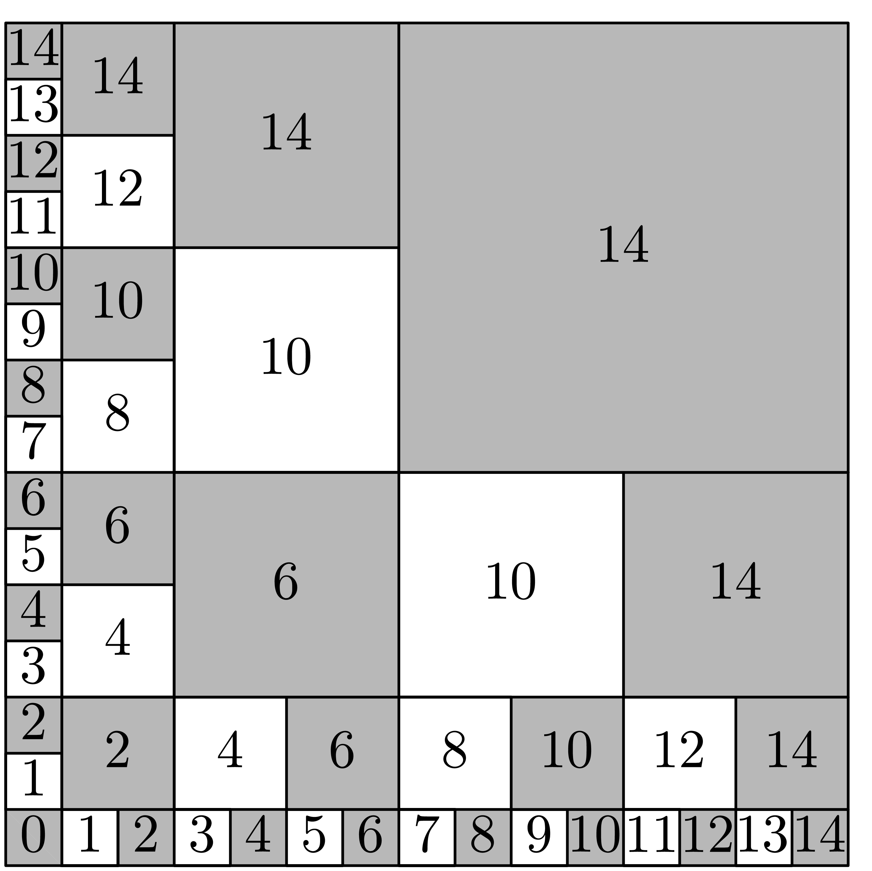
 where
where  ,
, ,
, ,
, ,
, .
.


 ,
, ,
,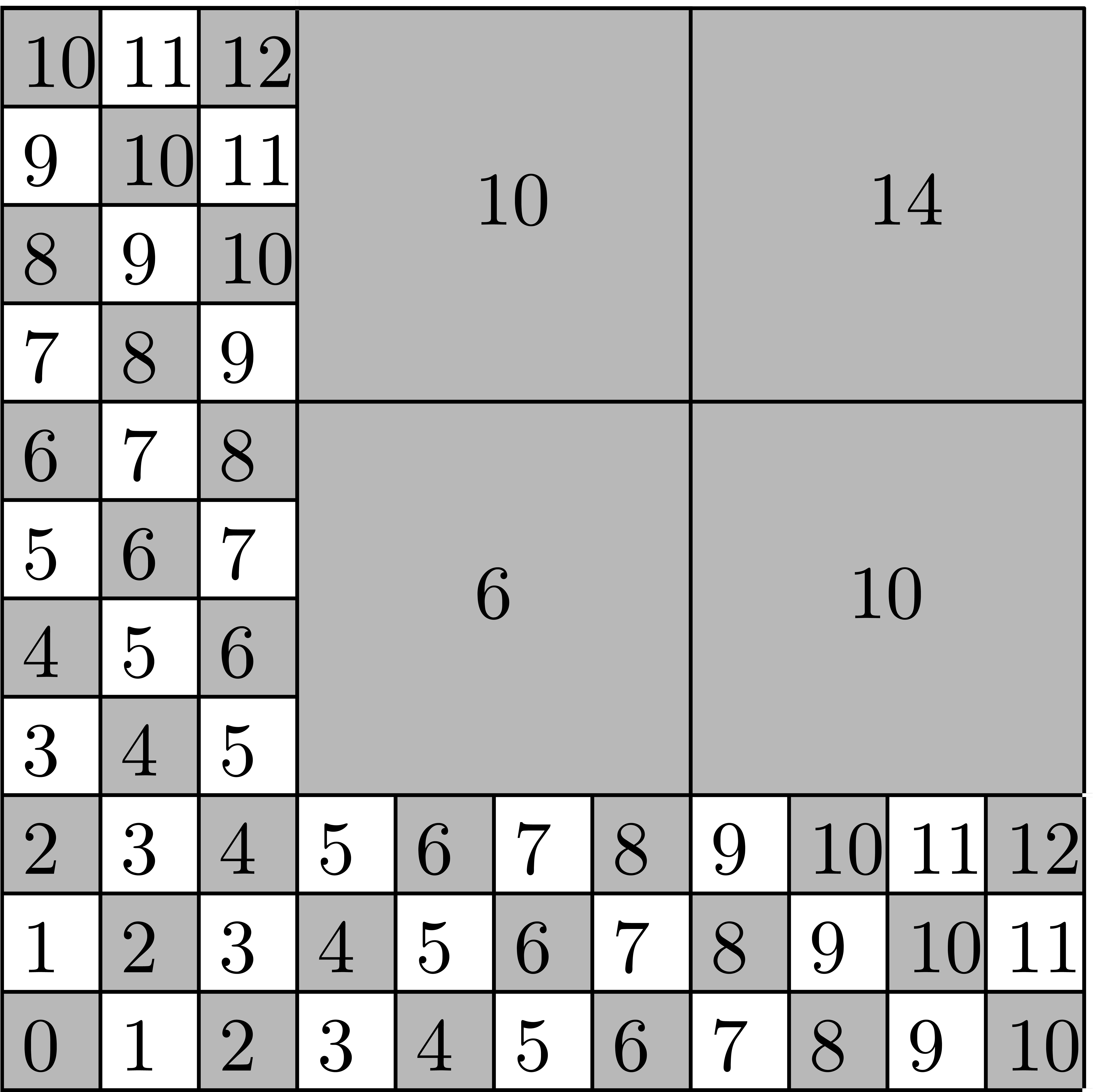
 and
and 


 ,
,


