Towards a library for straight-line programs

A straight-line program (or SLP) is a program that takes a finite number of input arguments, then executes a sequence of simple arithmetic instructions, and finally returns a finite number of output values. For instance, the function

can be computed using the following SLP:

The instructions operate on a finite list of variables (here

) and constants (here

). There are no restrictions on how variables are allowed to be reused: they can be reassigned several times (like

) and they may occur multiple times in the input and output of an operation (like in the operations

and

SLPs have a profoundly dual nature as programs and data. As programs, SLPs are eligible for a range of operations and techniques from the theory of compilation [3]: constant folding, common subexpression elimination, register allocation, etc. Although the expressive power of SLPs is very limited, their simplicity can be turned into an advantage: many program optimizations that are hard to implement for general purpose programs become simpler and more efficient when restricted to SLPs. In particular, most classical program transformations can be done in linear time. Traditional general purpose compilation techniques also rarely exploit mathematical properties (beyond basic algebraic rules that are useful during simplifications). In the SLP world, algebraic transformations such as automatic differentiation [14] and transposition [17] are easy to implement; more examples will be discussed in this paper.

Let us now turn to the data side. The example SLP (1.1) can be regarded as a polynomial

. In this sense, SLPs constitute a data structure for the representation of multivariate polynomials. Note that this representation is more compact than the (expanded) sparse representation

and way more compact than the dense “total degree” representation

. If our main goal is to evaluate a given polynomial many times, then the SLP representation tends to be particularly efficient. However, for explicit computations on polynomials, other representations may be preferred: for instance, the dense representation allows for FFT multiplication [40, section 8.2] and the sparse representation also allows for special evaluation-interpolation techniques [101].

The above efficiency considerations explain why SLPs have become a central framework in the area of algebraic complexity [21]. Joos Heintz has been an early proponent of polynomial SLPs in computer algebra. Together with Schnorr, he designed a polynomial time algorithm to test if an SLP represents the zero function or not, up to precomputations that only depend on the size of the SLP [55]. Later, Giusti and Heintz proposed an efficient algorithm to compute the dimension of the solution set of a system of homogeneous polynomials given by SLPs [43]. Then, Heintz and his collaborators showed that the polynomials involved in the Nullstellensatz had good evaluation properties, and could therefore be better represented by SLPs [47, 33] than by dense polynomials. These results led to a new method, called geometric resolution, which allows polynomial systems to be solved in a time that is polynomial in intrinsic geometric quantities [41, 44, 46, 51, 87].

In order to implement the geometric resolution algorithm, it was necessary to begin with programming efficient evaluation data structures. The first steps were presented at the TERA'1996 conference held in Santander (Spain) by Aldaz, and by Castaño, Llovet, and Martìnez [22]. Later on, a C++ implementation of SLPs was done by Hägele (a former PhD student of Heintz). Then another library was written in the Haskell language [20]. Independently, other experiments were conducted to implement the algorithm of [43] in the Maple computer algebra system, that was readily offering an evaluation data structure [42]. Further extensions of these approaches finally led to sharp complexity bounds and successful software implementations [48]. More references can be found in [30].

There are a few other concepts that are very similar to SLPs. Trees and directed acyclic graphs (DAGs) are other popular structures for the representation of mathematical expressions. Conversions to and from SLPs are rather straightforward, but SLPs have the advantage that they expose more low-level execution details. Since performance is one of our primary concerns, we therefore prefer the framework of SLPs in this paper.

Another related concept is the blackbox representation. Blackbox programs can be evaluated, but their “source code” is not available. This representation is popular in numerical analysis and the complexity of various numerical methods [98, Chapters 4, 9, 10, and 17] can be expressed in terms of the required number of function evaluations (the length of an SLP corresponds to the cost of one function evaluation in this context). The blackbox representation is also popular in computer algebra, especially in the area of sparse interpolation [81, 26, 101]. However, for programs that we write ourselves, it is unnatural to disallow opening the blackboxes. This restriction makes it artificially hard to perform many algebraic transformations such as modular reduction, automatic differentiation, etc. On the other hand, computing the determinant of an

matrix can easily be done in time

by a blackbox using Gaussian elimination. This task is less trivial for SLPs, since branching to find appropriate pivots is forbidden.

1.2.Design goals and overview of this paper

Despite the importance of SLPs for theoretical and practical purposes, they have not yet been the central target of a dedicated high performance library, up to our knowledge. (We refer to [36, 22, 20] for early packages for polynomial SLPs.) In contrast, such libraries exist for integer and rational numbers (Gmp [49]), multiple precision floating point numbers (Mpfr [35]), linear algebra (BLAS [15], Linbox [27]), ball arithmetic (Arb [76]), etc. As a consequence, we feel that a lot of potential advantages of SLPs are underexploited in current computer algebra systems and beyond.

In 2015, we started the development of such a dedicated library for SLPs, called Justinline. This library is part of the Mathemagix system [74] and publicly available via SVN since revision 10218. More recently, we have started a new reimplementation in C++ which aims at even higher performance. This new stand-alone library, called Jil, can be used with or without Mathemagix. Several of our past publications [70, 66] relied implicitly, but quite essentially, on the Justinline library. This paper focuses for the first time on the SLP libraries themselves. We will mainly present the high level motivations, goals, and design decisions. Future papers shall provide more details on the ongoing implementations and specific applications.

Performance is a primary motivation behind our work. Both operations on SLPs and their execution should be as efficient as possible. At the same time, we wish to be able to fully exploit the generality of the SLP framework. This requires a suitable representation of SLPs that is both versatile and efficient to manipulate. As will be detailed in section 2, we will represent SLPs using a suitable low-level encoding of pseudo-code as in (1.1), while allowing its full semantic richness to be expressed. For instance, the ordering of the instructions in (1.1) is significant, as well as the ability to assign values multiple times to the same variables. One may also specify a precise memory layout.

For instance, we might start with an SLP

that computes the determinant of a

matrix multiplication, then compute its gradient using automatic differentiation, then optimize this code, and finally generate executable machine code.

The initial SLP can be specified directly using low-level pseudo-code. But this is usually not most convenient, except maybe for very simple SLPs. In section 3, we describe a higher level recording mechanism. Given an existing, say, C++ template implementation for the computation of determinants of matrices, we may specialize this routine for a special “recorder” type and run it on a

matrix with generic entries. The recording mechanism will then be able to recover a trace of this computation and produce an SLP for determinants of

matrices.

In section 4, we turn to common program transformations like simplification, register allocation, etc. Although this is part of the classical theory of compilation, the SLP framework gives rise to several twists. Since our libraries are required to be very efficient, they allow us to efficiently generate SLPs on the fly. Such SLPs become disposable as soon as they are no longer needed. Consequently, our SLPs can be very large, which makes it crucial that transformations on SLPs run in linear time. The philosophy is to sacrifice expensive optimizations that require more time, but to make up for this by generating our SLPs in such a way that cheaper optimizations already produce almost optimal code. That being said, there remains a trade-off between speed of compilation and speed of execution: when a short SLP needs to be executed really often, it could still make sense to implement more expensive optimizations. But the primary focus of our libraries is on transformations that run in linear time.

When considering SLPs over specific algebraic domains such as integers, modular integers, floating point numbers, polynomials, matrices, balls, etc., it may be possible to exploit special mathematical properties of these domains in order to generate more efficient SLPs. This type of transformations, which can be problematic to implement in general purpose compilers, are the subject of section 5.

Popular examples from computer algebra are automatic differentiation [14] and transposition [17]. Another example was described in [70]: ball arithmetic allows us to lift any numerical algorithm into a reliable one that also produces guaranteed error bounds for all results. However, rounding errors need to be taken into account when implementing a generic ball arithmetic, which leads to a non-trivial overhead. When the algorithm is actually an SLP, this overhead can be eliminated through a static analysis. Similarly, assume given an SLP over arbitrary precision integers, together with a bound for the inputs. Then one may statically compute bounds for all intermediate results and generate a dedicated SLP that eliminates the need to examine the precisions during runtime. This may avoid many branches and subroutine calls.

Several applications that motivated our work are discussed in section 6. From the perspective of a high level application, the SLP library is a mixture of a compiler and a traditional computer algebra library. Instead of directly calling a high level function like a matrix product or a discrete Fourier transform (DFT), the idea is rather to compute a function that is able to efficiently compute matrix products or DFTs of a specified kind (i.e. over a particular coefficient ring and for particular dimensions). In this scenario, the library is used as a tool to accelerate critical operations.

High level master routines for matrix products and DFTs may automatically compile and cache efficient machine code for matrices and DFTs of small or moderate sizes. Products and DFTs of large sizes can be reduced to these base cases. It is an interesting question whether these master routines should also be generated by the SLP library. In any case, the SLP framework allows for additional flexibility: instead of statically instantiating C++ templates for a given type, we may generate these instantiations dynamically. Moreover, using the techniques from section 5, this can be done in a way that exploits mathematical properties of the type, which are invisible for the C++ compiler.

More specifically, we will discuss applications to numerical homotopy continuation, discrete Fourier transforms, power series computations, differential equations, integer arithmetic, and geometric resolution of polynomial systems. There are many other applications, starting with linear algebra, but our selection will allow us to highlight various particular advantages and challenges for the SLP framework.

The last section 7 is dedicated to benchmarks. Some timings for the Justinline library were already presented in our previous papers [70, 66]. For this reason, we mainly focus on some first timings for the Jil library, while noting that the development of this library is still at an early and experimental stage. Nonetheless, we were able to appreciate a significant speed-up for operations on SLPs with respect to the Justinline library; the generated machine code is of comparable quality.

Acknowledgments. We wish to thank Albin Ahlbäck, Alexander Demin, and Arnaud Minondo for useful discussions and suggestions.

2.The SLP data type

2.1.Abstract SLPs

We start this section with an abstract formalization of SLPs. Our presentation is slightly different from [21] or [70], in order to be somewhat closer to the actual machine representation that we will describe next.

Let

be a set of operation symbols together with a function

. We call

a signature and

the arity of

, for any operation

. A domain with signature

is a set

together with a function

for every

. We often write

instead of

if no confusion can arise. The domain

is said to be effective if we have data structures for representing the elements of

and

on a computer and if we have programs for

and

, for all

Example 2.1. For the introductory example (1.1), we may take

to be the signature of rings with

and

to be the ring

Remark 2.2. In model theory and mathematical logic,

is also called a language (without relation symbols) and

a structure for this language; see, e.g., [7, Appendix B]. For simplicity, we restricted ourselves to one-sorted languages, but extensions to the multi-sorted case are straightforward.

with

and arguments

, where

. We call

the destination argument or operand and

the source arguments or operands. We denote by

the set of such instructions. Given

, we also let

. A straight-line program (SLP) over

is a quadruple

, where

We regard

as the working space for our SLP. Each location in this working space can be represented using an integer in

and instructions directly operate on the working space as we will describe now.

Given a state

of our working space, the execution of an instruction

gives rise to a new state

where

and

. Given input values

, the corresponding begin state

of our SLP is given by

and

for

. Execution of the SLP next gives rise to a sequence of states

. The output values

of our SLP are now given by

for

. In this way our SLP

gives rise to a function

that we will also denote by

. Two SLPs will be said to be equivalent if they compute the same function.

Example 2.3. With

and

as in Example 2.1, our introductory example (1.1) can be represented as follows:

, and

with

One may check that this SLP indeed computes the intended function when using the above semantics. Note that we may chose arbitrary values for the input fields

, the output field

, and the auxiliary data fields

. So we may just as well take them to be zero, as we did.

For the sake of readability, we will continue to use the notation (1.1) instead (2.1), the necessary rewritings being clear. If we wish to make the numbering of registers precise in (1.1), then we will replace

Note that

is not really an instruction, but rather a way to indicate that the data field

contains the constant

It will be useful to call elements of

variables and denote them by more intelligible symbols like

whenever convenient. The entries of

and

are called input and output variables, respectively. Non-input variables that also do not occur as destination operands of instructions in

are called constants. An auxiliary variable is a variable that is neither an input variable, nor an output variable, nor a constant. Given a variable

the corresponding data field is

. Input variables, output variables, and constants naturally correspond to input fields, output fields, and constant fields.

Remark 2.4. One might prefer to use mutually distinct input variables, output variables, auxiliary variables, and constants. One may also wish to impose that output variables can only be assigned once. In our formalism none of this is mandatory, but any SLP can easily be rewritten into an equivalent SLP that satisfies these properties. The ability to share input and output variables or different output variables can be useful in order to keep the length

of the SLP as small as possible.

Remark 2.5. Testing the equivalence of two polynomial SLPs is hard in general [80]. But there is an easy probabilistic algorithm to do this: simply evaluate the SLP at a random point. For SLPs of bounded size, Heintz and Schnorr showed how to derandomize this method, by using a suitable deterministic sequence of points instead [55]. Of course, this only works in theory, since such sequences are necessarily hard to compute!

2.2.Choice of the signature

One crucial design decision concerns the choice of the signature

and the way how operations are represented.

On the one hand, we do not want to commit ourselves to one specific signature, so it is important to plan future extensions and even allow users to specify their own dynamic signatures. This kind of flexibility requires no extra implementation effort for many “signature-agnostic” operations on SLPs, such as common subexpression elimination, register allocation, etc. On the other hand, the precise signature does matter for operations like simplification, automatic differentiation, etc. We need our code to be as efficient as possible for the most common operations in

, while providing the possibility to smoothly extend our implementations to more exotic operations whenever needed.

In the Justinline library, we chose to represent the operations in

by abstract expressions. Exploiting pattern matching facilities inside Mathemagix, this allowed us to implement operations on SLPs in an elegant and naturally extensible way. However, this design choice resulted in a non-trivial efficiency overhead. In the Jil library, we therefore decided to represent operations more directly by machine integers. Some of the bits of these integers are reserved for interesting properties of the operation, such as its arity. Lookup tables are used to retrieve more extensive information.

What about the choice of a subsignature

of operations that we deem to be “most common” and that should benefit from particularly efficient support in the library? At the end of the day, we wish to turn our SLPs into efficient machine code. It is therefore useful to draw inspiration from the instruction sets of modern CPUs and GPUs. For example, this motivated our decision to include the fused multiply add (FMA) operation

, together with its signed variants

, and

. Although this adds to the complexity of

(why not emulate FMA using multiplication and addition?), this decision tends to result in better machine code (more about this below; see also section 5.7).

However, the instructions sets of modern processors are very large. In order to keep our SLP library as simple as possible, it would be unreasonable to directly support all these instructions. Much of the complexity of modern instruction sets is due to multiple instances of the same instruction for different data types, SIMD vector widths, immediate arguments, addressing modes, guard conditions, etc. In the SLP setting it is more meaningful to implement general mechanisms for managing such variants. Modern processors also tend to provide a large number of exotic instructions, which are only needed at rare occasions, and which can typically be emulated using simpler instructions.

One useful criterion for deciding when and where to support particular operations is to ask the question how easily the operation can be emulated, while resulting in final machine code of the same quality. Let us illustrate this idea on a few examples.

Imagine that our hardware supports FMA, but that we did not include this operation in

. In order to exploit this hardware feature, we will need to implement a special post-processing transformation on SLPs for locating and replacing pairs of instructions like

and

by FMAs, even when they are separated by several independent instructions. This is doable, but not so easy. Why bother, if it suffices to add FMA to our signature and generate high quality code with FMAs from the outset? Maybe it will require more implementation efforts to systematically support FMAs inside our routines on SLPs, but we won't need a separate and potentially expensive post-processing step.

In fact, for floating point numbers that follow the IEEE 754 standard [5], the FMA instruction cannot be emulated using one multiplication and one addition. This is due to the particular semantics of correct rounding: if

denotes the double precision number that is nearest to a real number

, then we do not always have

. The IEEE 754 rounding semantics can be exploited for the implementation of extended precision arithmetic [25, 99, 69, 77] and modular arithmetic [13, 73]. This provides additional motivation for including FMA in our basic signature

We do not only have flexibility regarding the signature

, but also when it comes to the domains

that we wish to support. For the selection of operations in

, it is also important to consider their implementations for higher level domains, such as modular integers, matrices, truncated power series, etc. Now the implementation of

is often simpler than the combined implementation of

and

. For instance, if

is the domain of

matrices over a field, then

can be implemented using

FMAs over

, whereas its emulation via

and

would require

instructions. One may argue that the better code should be recoverable using a suitable post-processing step as described above. This is true for matrix multiplication, but turns out to become more problematic for other domains, such as modular integers that are implemented using floating point FMAs. Once more, the inclusion of FMA into our signature

tends to facilitate the generation of high quality machine code.

Let us finish with an example of some operations that we do not wish to include in

. Instruction sets of CPUs allow us to work with integers and floating point numbers of various precisions. How can we do computations with mixed types in our framework? Instead of mimicking the CPUs instruction set within

, the idea is rather to provide a general mechanism to dynamically enrich

. Here we may exploit the fact that our framework made very few assumptions on

and

. Given domains

of signatures

, the idea is to dynamically create a signature

and a domain

such that

operates on

via

and

otherwise. We regard

and

as being disjoint, which allows us to dynamically add

In this way, it is easy to emulate computations with mixed types and signatures in our abstract SLP framework (and thereby support multi-sorted structures as in Remark 2.2). This kind of emulation comes with some overhead though. But we consider this to be a small price to pay for the simplicity that we gain by avoiding the management of multiple types and signatures in the framework itself.

2.3.Representation of domains

The SLP framework is more general than it may seem at first sight due to the fact that we are completely free to chose the signature

and the underlying domain

. In principle, this allows for all data types found in computer algebra systems. Nonetheless, for our library it is wise to include privileged support for a more restricted set of domains, similarly to what we did with

in the case of signatures.

First of all, we clearly wish to be able to have domains for all the machines types that can be found in hardware. In traditional CPUs, these types were limited to floating point numbers and (signed and unsigned) integers of various bit-sizes. In modern CPUs and GPUs, one should add SIMD vector versions of these types for various widths and possibly a few more special types like matrices and polynomials over

of several sizes and degrees.

On top of the machine types, we next require support for basic arithmetical domains such as vectors, matrices, polynomials, jets, modular integers and polynomials, extended precision numbers, intervals, balls, etc. Such functionality is commonplace in computer algebra systems or specialized HPC libraries such as Flint [53]. However, in the Justinline and Jil libraries, special attention is paid to domains for which the corresponding signature can itself be implemented using SLPs over lower level types. We call such domains SLP algebras and we will describe them in more detail in section 5.5 below. The domain

matrices with 64 bit integer coefficients in a typical example of an SLP algebra. One advantage is that instances can always be represented as dense vectors of a fixed size.

In the Justinline library, we implemented SLPs as a type that is templated by the domain. Here we take advantage of the fact that Mathemagix supports both static templates (that are instantiated at compile time, like in C++) and dynamic templates (for which the template parameters are passed as extra parameters); see [68, 67]. Template parameters are themselves typed, which means that the signature

of our domain must be specified. In our implementation, we use

as the signature, while agreeing that operations in

that are not implemented for a given domain simply raise an error. We also provide default implementations for operations like FMA that can be emulated using other operations. In order to achieve full extensibility, it suffices to add a generic operation to our signature for all operations in

; the arguments of this generic operation are the concrete operation in

and the (variable number of) arguments of this operation.

In our lower level C++ implementation in Jil, we introduced a special abstract data type domain for domains. Each operation in

gives rise to a virtual method for this type which can carry out the operation for the concrete domain at hand. An element of a domain is represented as one consecutive block of data inside memory. The size of this block is fixed and can be retrieved using another virtual method of the domain type. This mechanism is essentially the same as the one from the Justinline library, except that static instantiation for a particular domain is no longer possible (of course, this leads to some overhead, but we will see in section 3 below that this will usually not be a problem, because our real aim will be to record execution traces). Full extensibility can again be achieved by adding one more virtual function for generic operations.

2.4.Low-level representation of SLPs

Given an abstract SLP

, it is natural to represent

, and

as actual vectors in contiguous memory. In the cases of

and

, these vectors have machine integer coefficients. If elements of

can themselves be represented by vectors of a fixed size, then one may use the additional optimization to concatenate all entries of

into a single vector, which we do in the Jil library.

For the representation of programs

, we have several options. In the Justinline library, we use a separate data type for instructions in

, so that

is simply represented as a vector of instructions. In Jil, both elements of

and the arguments of instructions are represented by machine integers. Consequently, instructions in

can be represented by machine integer vectors. This again makes it possible to concatenate all instructions into a single machine integer vector, which can be thought of as “byte code”.

The systematic concatenation of vector entries of vectors in Jil greatly reduces the number of memory allocations. Note however that instructions may have different lengths as vectors. If we wish to quickly address specific instructions, one linear pass through

is required in order to build a table with the offsets of the individual instructions. Alternatively, we could have imposed a maximal arity for the operations in

, which would have allowed us to represent all instructions by vectors of the same length. This alternative representation is less compact but has the advantage that individual instructions can be addressed more easily. It is also not so clear what would be a good maximal arity.

The Jil library contains one more low-level optimization. Instructions and data fields of SLPs are typically built one by one. During their construction, this means that

and

should really be considered as output streams rather than vectors. Moreover, it is almost always possible to give a simple and often tight a priori bound for the lengths of

and

at the end of this streaming process. This makes it possible to allocate these vectors once and for all and directly stream the entries without being preoccupied by range checks or reallocations of larger memory blocks.

We have considered but discarded a few alternative design options. All operations in

have a single output value in our implementation. Since SLPs are allowed to have multiple output values, it might be interesting to allow the same thing for operations in

. Some instructions in CPUs are indeed of this kind, like long multiplication (x86) or loading several registers from memory (ARM). However, this elegant feature requires an additional implementation effort for almost all operations on SLPs. This also incurs a performance penalty, even for the vast majority of SLPs that do not need this feature.

Note finally that it is still possible to emulate instructions with multiple outputs by considering single vector outputs and then introducing extra instructions for extracting entries of these vectors. Unfortunately however, this is really inelegant, because it forces us to use more convoluted non-fixed-sized vector domains. It is also non-trivial to recombine these multiple instructions into single machines instruction when building the final machine code.

Similar considerations apply for in-place semantics like in the C instruction a+=b. Here again, we note that our SLP formalism allows for this kind of semantics, since entries of

and

are not required to be disjoint. But it is also easy to emulate an instruction like a+=b by a=a+b.

Yet another interesting type of alternative design philosophy would be to systematically rule out redundant computations by carrying out common subexpression elimination during the very construction of SLPs. However, for cache efficiency, it is sometimes more efficient to recompute a value rather than retrieving it from memory. Our representation provides greater control over what is stored where and when. The systematic use of common subexpression elimination through hash tables also has a price in performance.

2.5.On the quality of SLPs

Recall that two SLPs are equivalent if they compute the same mathematical function. Among two equivalent SLPs, the shorter one is typically most efficient. But the length of an SLP is not the only factor for its practical performance. It is also important to keep an eye on dependency chains, data locality, and cache performance. Besides performance, “readability” of an SLP may also be an issue: we often change the numbering of data fields in a way that makes the SLP more readable.

We catch all these considerations under the concept of quality. This concept is deliberately vague, because the practical benefits of SLPs of “higher quality” depend greatly on our specific hardware. Operations on SLPs should be designed carefully in order to avoid needless quality deteriorations. This can often be achieved by touching the input SLPs “as least as possible” and only in “straightforward ways”.

Let us briefly review how dependency chains and data layout may affect the performance. Consider the following two SLPs for complex multiplication:

Here

stands for “fused multiply subtract” and

for “fused multiply add”. Modern hardware tends to contain multiple execution units for additions, multiplications, fused multiplications, etc., which allow for out of order execution [75, 6, 34]. In the right SLP, this means that the instruction

can be dispatched to a second multiplication unit while

is still being executed by a first unit. However, in the left SLP, the instruction

has to wait the for the outcome of

. Whereas the fused multiplications in both SLPs depend on the result of one earlier multiplication, these dependencies are better spread out in time in the right SLP, which typically leads to better performance.

Let us now turn to the numbering of our data fields in

. When generating the final machine code for our SLP, we typically cut

into a small number of contiguous blocks, which are then mapped into contiguous chunks in memory. For instance, we might put the input, output, auxiliary, and constant fields in successive blocks of

and map them to separate chunks in memory.

Now memory accesses are most efficient when done per cache line. For instance, if cache lines are 1024 bits long and if we are working over 64 bit double precision numbers, then fetching

from memory will also fetch

. The cache performance of an SLP will therefore be best when large contiguous portions of the program

access only a proportionally small number of data fields

, preferably by chunks of 16 contiguous fields. The theoretical notion of cache oblivious algorithms [39] partially captures these ideas. Divide and conquer algorithms tend to be cache oblivious and thereby more efficient. Computing the product of two

matrices using a naive triple loop is not cache oblivious (for large

) and can therefore be very slow. In the terminology of this subsection, high quality SLP should in particular be cache oblivious.

3.Recording SLPs

Where does the “initial SLP”

come from in the workflow (1.2)? It is not very convenient to oblige users to specify

using pseudo-code like (1.1), (2.1), or (2.2). Now we often already have some existing implementation of

, albeit not in our SLP framework. In this section we explain how to derive an SLP for

from an existing implementation, using a mechanism that records the trace of a generic execution of

Modulo the creation of appropriate wrappers for recording, this mechanism applies for any existing code in any language, as long as the code is either generic or templated by a domain

that implements at most the signature

. By “at most”, we mean that the only allowed operations on elements from

are the ones from

Recording can be thought of as a more powerful version of inlining, albeit restricted to the SLP setting: instead of using complex compilation techniques for transforming the existing code, it suffices to implement a cheap wrapper that records the trace of an execution. Hence the names Justinline and Jil.

3.1.Recorder types

Let us describe how to implement the recording mechanism for existing C or C++ code over a domain

. For this we introduce a type recorder, which could either be a template with

as a parameter, or a generic but slower recorder type that works over all domains. In order to record a function, say

, we proceed as follows:

slp
record_f () {
  start_recorder ();
  recorder in1= input ();
  recorder in2= input ();
  recorder out= f (in1, in2);
  output (out);
  return stop_recorder ();
}

In this code we use global variables for the state of the recorder. This state mainly consists of the current quadruple

, where

are thought of as output streams (rather than vectors).

When starting the recorder, we reset

to being empty. Instances of the recorder type represent indices of data fields in

The instruction in1=input() adds a new zero element to

, adds the corresponding index (

in this case) to

, and next stores it in in1. Similarly, the code in2=input() adds a second zero element to

, adds the corresponding index

, and then stores it in in2.

We next execute the actual function

on our input data. For this, the data type recorder should implement a default constructor, a constructor from

, and the operations from

(as well as copy and assignment operators to comply with C++). The default constructor adds a new auxiliary data field to

, whereas the constructor from

adds a new constant field. An operation like multiplication of

and

creates a new auxiliary destination field

and streams the instruction

into

At the end, the instruction output(out) adds out to

and stop_recorder() returns the SLP represented by the quadruple

Remark 3.1. The above implementation introduces a new auxiliary data field for every operation. This results in SLPs that use more data fields than necessary. Let us describe how to improve this. First of all, we now represent instances of recorder by an index, as before, together with a flag that indicates whether the instance corresponds to an auxiliary field or to an input, output, or constant field. We next create a destructor for recorder: whenever we destroy an auxiliary field, we add its index to a stack. This stack of destroyed data fields is maintained as part of the global state and emptied when calling start_recorder. We next adapt the default constructor of auxiliary fields to reclaim them from the stack and only introduce a new data field when the stack is empty.

Remark 3.2. When the same constant is constructed multiple times during the execution of

, the above recording algorithm will put them in separate data fields. Another useful optimization is to maintain a table of constants (as part of the global state) and directly reuse constants that where allocated before.

3.2.Recording

matrix multiplication

Let us investigate in detail what kind of SLPs are obtained through recording on the example of

matrix multiplication. Assume that matrices are implemented using a C++ template type matrix<C> with the expected constructors and accessors. Assume that matrix multiplication is implemented in the following way:

template<typename C> matrix<C>
operator * (const matrix<C>& M, const matrix<C>& N) {
  int r= rows (M), l= columns (M), c= columns (N);
  if (rows (N) != l) throw "error";
  matrix<C> R (r, c);
  for (int i=0; i<r; i++)
    for (int (j=0; j<c; j++) {
      C sum= 0;
      for (int k=0; k<l; k++)
        sum= sum + M(i,k) * N(k,j);
      R(i,j)= sum;
    }
  return R;
}

When applying this code for two generic

input matrices in a similar way as in the previous subsection, without the optimizations from Remarks 3.1 and 3.2, we obtain the following SLP:

(The order of this code is column by column from left to right.) In order to understand the curious numbering here, one should remind how constructors work: the declaration of R gives rise to four default constructors of instances of recorder. These are put in

but never used. The constructor of sum next creates the constant

, which is put in

. We then record the successive instructions, the results of which are all put in separate data fields. Note that

are not really instructions, but rather a convenient way to indicate the constant fields

all contain zero.

When applying the optimizations from Remarks 3.1 and 3.2, the generated code becomes as follows:

The numbering may look even odder (although we managed to decrease the length of

). This is due to the particular order in which auxiliary data fields are freed and reclaimed via the stack.

3.3.Towards the direct generation of cleaner code

The example from the previous subsection shows that the recording mechanism does not generate particularly clean SLPs. This is not per se a problem, because right after recording a function we typically simplify the resulting SLP, as will be detailed in section 4.4 below. However, the simplifier may not be able to correct all problems that we introduced when doing the recording in a naive manner. Simplification also tends to be faster for shorter and cleaner SLPs. Simplification might not even be needed at all.

The advantage of the mechanism from the previous section is that it can be applied to an external template C++ library over which we have no control. One reason for the somewhat messy results (3.1) and (3.2) is that C++ incites us to create classes with nice high level mathematical interfaces. Behind the scene, this gives rise to unnecessary temporary variables and copying of data. We may avoid these problems by using a lower level in-place interface for C and matrix<C>. For instance:

template<typename C> void
mul (matrix<C>& R, const matrix<C>& M, const matrix<C>& N) {
  int r= rows (M), l= columns (M), c= columns (N);
  if (rows (N) != l || rows (R) != r || columns (R) != c)
    throw "error";
  for (int i=0; i<r; i++)
    for (int (j=0; j<c; j++) {
      mul (R(i,j), M(i,0), N(0,j));
      for (int k=1; k<l; k++)
        fma (R(i,j), M(i,k), N(k,j), R(i,j));
    }
}

When recording our SLP using this kind of code, we obtain a much cleaner result:

For this reason, the Jil library implements various common domains (vectors, matrices, polynomials, modular numbers, balls, etc.) using an in-place style. As explained in section 2.3, this implementation is generic, which induces a performance penalty with respect to the above template implementation. But this does not really matter: the focus of our generic implementation is not on high execution speed, but on the generation of high quality SLPs through recording. At a second stage, we will be able to generate even more efficient machine code from these SLPs.

Remark 3.3. The in-place calling convention comes with the subtlety that destination arguments might collide with source arguments. This phenomenon, called aliasing, is both a pain and a blessing.

It is a pain because the above multiplication algorithm becomes incorrect in this situation. Fortunately there is the easy remedy to copy colliding arguments into auxiliary variables. Testing for collisions induces additional overhead when recording the code, but the generated SLP is not impacted if no collisions occur.

What is more, if collisions do occur, then we actually have the opportunity to generate an even better SLP. This is for instance interesting for discrete Fourier transforms (DFTs), which can either be done in-place or out-of-place. In our framework, we may implement a single routine which tests in which case we are and then uses the best code in each case.

3.4.A shifted design perspective

The shifted perspective from efficiency of execution to quality of recorded code cannot be highlighted enough.

One consequence is that the overhead of control structures only concerns the cost of recording the SLP, but not the cost of executing the SLP itself. For example, in Remark 3.3, this holds for the cost of checking whether there are collisions between input and output arguments. But the same holds for the overhead of recursive function calls. For instance, one may implement matrix multiplication recursively, by reducing an

product into an

and an

product with

and

(or using a similar decomposition for

if these are larger). The advantage of such a recursive strategy is that it tends to have a better cache efficiency. Now traditional implementations typically recurse down only until a certain threshold, like

, because of the overhead of the recursive calls. But this overhead disappears when the multiplication is recorded as an SLP, so we may just as well recurse down to

An even more extreme example is relaxed power series arithmetic. Consider basic arithmetic operations on truncated power series such as inversion, exponentiation, etc. If the series are truncated at a fixed order

that is not too large (say

), then lazy or relaxed algorithms are particularly efficient (see [57] and section 6.3 below). However, they require highly non-conventional control structures, which explains that they are not as widely used in computer algebra systems as they might be. This disadvantage completely vanishes when these operations are recorded as SLPs: there is still a little overhead while recording an SLP, but not when executing it.

The shifted perspective means that we should focus our attention on the SLP that we wish to generate, not on the way that we generate it. For instance, the SLP (3.3) is still not satisfactory, because it contains several annoying dependency chains: the execution of the instruction

cannot start before completing the previous instruction

and similarly for the other FMAs. For CPUs with at least 12 registers, the following SLP would behave better:

Again, the SLP (3.3) could have been rewritten into this form automatically, using an appropriate optimization that detects dependency chains and reschedules instructions. Another observation is that the dependency chains were not present in (3.1), so they were introduced by the optimizations from Remark 3.1; this problem can be mitigated by replacing the first-in-first-out “stack allocator” by one that disallows the last

freed registers to be immediately reused. But then again, it is even better to design the routines that we wish to record in such a way that none of these remedies are needed. For instance, when doing

matrix products in the above recursive fashion, it suffices to recurse on

when

and

The Jil library comes with additional tools to ease programming according to this “shifted design perspective”: an abstract type map for maps (and intended to be optimized for recording), abstract types object and ref for data objects and references (that make it easy to access data structures in a strided way, for instance), and more. We plan to detail these more advanced features in future work.

4.Traditional operations on SLPs

This section is dedicated to classical program transformations like common subexpression elimination, simplification, register allocation, etc. As explained in the introduction, this is part of the traditional theory of compilation, but the SLP framework gives rise to several twists. SLPs can become very large and should therefore be disposable as soon as they are no longer needed. Our resulting constraint is that all algorithms should run in linear time (or in expected linear time if hash tables are required).

We recall that another important general design goal is to preserve the “quality” of an SLP as much as possible during transformations. The example SLPs (3.1), (3.2), (3.3), and (3.4) from the previous subsection are all equivalent, but their quality greatly differs in terms of code length, data locality, cache efficiency, dependency chains, and general elegance. It is the responsibility of the user to provide initial SLPs of high quality in (1.2). But it is on the SLP library to not deteriorate this quality during transformations, or, at least, to not needlessly do so. An extreme case of this principle is when the input SLP already accomplishes the task that a transformation is meant to achieve. Ideally speaking, the transformation should then simply return the input SLP. One typical example is the simplification of an already simplified SLP.

4.1.Extracting basic information

For the sake of completeness, we first describe with some very basic and straightforward operations on SLPs that are essentially related to their representation. These operations are often used as building blocks inside more complex transformations.

We start with the extraction of useful information about a given SLP. Concerning the variables in

, we may build boolean lookup tables of length

for the following predicates:

We may also build lookup tables to collect information about the program

itself. Let us focus on Jil and recall that we use “byte code”

for the internal low level representation of

. Every instruction

thus corresponds to a part of the byte code: for some offset

(with

and

otherwise), we have

. For this representation, the following information is typically useful:

Clearly, all these types of information can easily be obtained using one linear pass through the program

4.2.Tweaking the representation

We discussed several design options for the representations of SLPs in section 2. The options that we selected impose few restrictions, except for the one that all instructions have a single destination operand. This freedom allows us to express low level details that matter for cache efficiency and instruction scheduling. However, it is sometimes useful to impose additional constraints on the representation. We will now describe several basic operations on SLPs for this purpose.

The function computed by an SLP clearly does not depend on the precise numbering of the data fields in

. If the input and output variables are pairwise distinct, then we may always impose them to be numbered as

and

: for this it suffices to permute the data fields.

Similarly, we may require that all variables actually occur in the input, the output, or in the program

itself: if

are the variables that occur in the SLP, then it suffices to renumber

into

, for

. When applied to the SLP from (3.1), we have

for

and

for

, so we suppress

useless data fields.

A stronger natural condition that we may impose on an SLP is that every instruction participates in the computation of the output. This can be achieved using classical dead code optimization, which does one linear pass through

in reverse direction. When combined with the above “dead data” optimization, we thus make sure that our SLPs contain no obviously superfluous instructions or data fields.

Our representation of SLPs allows the same variables to be reassigned several times. This is useful in order to reduce memory consumption and improve cache efficiency, but it may give rise to unwanted dependency chains. For instance, the SLP (3.2) contains more dependency chains than (3.1): the instruction

must be executed before

, but the instructions

and

can be swapped. In order to remove all dependency chains due to reassignments, we may impose the strong condition that all destination operands in our SLP are pairwise distinct. This can again easily be achieved through renumbering. Note that the non-optimized recording strategy from section 3.1 has this property.

In Remark 3.3, we discussed the in-place calling convention that is allowed by our formalism and we saw that aliasing may negatively impact the correctness of certain algorithms. For some applications, one may therefore wish to forbid aliasing, which can easily be achieved through numbering. This can be strengthened further by imposing all input and output variables

to be pairwise distinct.

4.3.Common subexpression elimination

A powerful optimization in order to avoid superfluous computations is common subexpression elimination (CSE). The result of each instruction in

can be regarded as a mathematical expression in the input variables of our SLP. We may simply discard instructions that recompute the same expression as an earlier instruction. In order to do this, it suffices to build a hash table with all expressions that we encountered so far, using one linear pass through

In our more algebraic setting, this mechanism can actually be improved, provided that our domain

admits an algebraic hash function. Assume for instance that

and let

be a large prime number. Let

be the arguments of the function computed by our SLP and let

be uniformly random elements of

, regarded as a subset of the finite field

. Given any polynomial expression

, we may use

as an algebraic hash value for

. The probability that two distinct expressions have the same hash value is proportional to

, and can therefore be made exponentially small in the bit-size of

and the cost of hashing.

When using this algebraic hash function for common subexpression elimination (both for hashing and equality testing), mathematically equivalent expressions (like

and

) will be considered as equal, which may result in the elimination of more redundant computations. However, this algorithm is only “Monte Carlo probabilistic” in the sense that it may fail, albeit with a probability that can be made arbitrarily (and exponentially) small. Due to its probabilistic nature, we do not use this method by default in our libraries. The approach also applies when

, in which case divisions by zero (in

but not in

) only arise with exponentially small probability.

When implementing CSE in a blunt way, it is natural to use a separate data field for every distinct expression that we encounter. However, this heavily deteriorates the cache efficiency and reuse of data in registers. In order to preserve the quality of SLPs, our implementation first generates a blunt SLP with separate fields for every expression (but without removing dead code). This SLP has exactly the same shape as the original one (same inputs, outputs, and instructions, modulo renumbering). During a second pass, we renumber the new SLP using numbers of the original one, and remove all superfluous instructions.

4.4.Simplification

Simplification is an optimization that is even more powerful than common subexpression elimination. Mathematically speaking, an SLP always computes a function, but different SLPs may compute the same function. In particular, the output of CSE computes the same function as the input. But there might be even shorter and efficient SLPs with this property.

In full generality, finding the most efficient SLP for a given task is a difficult problem [21, 103, 93]. This is mainly due to the fact that an expression may first need to be expanded before an actual simplification occurs:

In our implementation, we therefore limited ourselves to simple algebraic rules that never increase the size of expressions and that can easily be applied in linear time using a single pass through the input SLP:

Simplification is a particularly central operation of the Justinline and Jil libraries: we typically apply simplification directly after recording, automatic differentiation, and various other high level routines on SLPs. Efficiency is therefore a firm constraint. Note that our simplification procedures also comprise CSE.

In the Jil library, we also “harmonized” the set

of basic operations with the set of simplification rules by introducing all possible versions of signed multiplication: besides the four versions

of signed FMAs, our signature

also contains the operation

. The resulting uniform treatment of signs is particularly beneficial for complex arithmetic, linear algebra (when computing determinants), polynomial and series division, automatic differentiation, and various other operations that make intensive use of signs.

4.5.Register allocation

Just before generating machine code for our SLP in the workflow (1.2), it is useful to further “massage” our SLP while taking into account specific properties of the target hardware. Register allocation is a particularly crucial preparatory operation.

Consider a target CPU or GPU with

registers. In our SLP formalism, the goal of register allocation is to transform an input SLP into an equivalent SLP with the following properties:

In our implementations, we also assume that

for all input/output variables and constants, but this constraint can easily be relaxed if needed.

There is a rich literature on register allocation. The problem of finding an optimal solution is NP-complete [24], but practically efficient solutions exist, based on graph coloring [24, 23, 19] and linear scanning [96]. The second approach is more suitable for us, because it is guaranteed to run in linear time, so we implemented a variant of it.

More precisely, using one linear pass in backward direction, for each operand of an instruction, we first determine the next location where it is used (if anywhere). We next use a greedy algorithm that does one more forward pass through

. During this linear pass, we maintain lookup tables with the correspondence between data fields and the registers they got allocated to. Whenever we need to access a data field that is not in one of the registers, we search for a register that is not mapped to a data field or whose contents are no longer needed. If such a register exists, then we take it. Otherwise, we determine the register whose contents are needed farthest in the future. We then save its contents in the corresponding data field, after which the register becomes available to hold new data.

This simple strategy efficiently produces reasonably good (and sometimes very good) code on modern hardware. In the future, we might still implement some of the alternative strategies based on graph coloring, for cases when it is reasonable to spend more time on optimization.

The complexity of our current implementation is bounded by

, because we loop over all registers whenever we need to allocate a new one. The dependence on

could be lowered to

by using heaps in order to find the registers that are needed farthest in the future. This optimization would in fact be worth implementing: for very large SLPs, one may regard different L1 and L2 cache levels as generalized register files. It thus makes sense to successively apply register allocation for, say,

, and

. The efficiency of this optimization might be disappointing though if our SLP does not entirely fit into the instruction cache: in that case the mere execution of the SLP will become a major source of cache misses.

Unfortunately, the above simple allocation strategy is not always satisfactory from the dependency chain point of view. For instance, consider the evaluation of a constant dense polynomial of high degree

using Horner's rule. The greedy algorithm might systematically reallocate the last

constant coefficients to same register. This unnecessarily puts a “high pressure” on this register, which results in unnecessary dependencies. The remedy is to pick a small number

, say

, and blacklist the last

allocated registers from being reallocated. As a result, the pressure will be spread out over

registers instead of a single one.

Remark 4.1. ARM CPUs only support register arguments for arithmetic instructions. On X86 processors, many instructions allow for one indirect memory argument. In that case, we can release our requirement that all instructions except “move” only accept register arguments.

4.6.Instruction scheduling

Both SLPs are equivalent and compute the sums

and

. However, the first SLP contains two long dependency chains of length

, whereas these dependency chains got interleaved in the second SLP.

Modern CPUs contain multiple execution units for addition. This allows the processor to execute the instructions

and

in parallel for

, as well as the first instructions

and

. Modern hardware has also become particularly good at scheduling (i.e. dispatching instruction to the various execution units): if

is not so large, then the execution of

in the first SLP may start while the execution of

is still in progress. However, processors have a limited “look-ahead capacity”, so this fails to work when

exceeds a certain threshold. In that case, the second SLP may be executed almost twice as fast, and it may be desirable to find a way to automatically rewrite the first SLP into the second one.

A nice way to accomplish this task is to emulate what a good hardware scheduler does, but without being limited by look-ahead thresholds. For this, we first need to model our hardware approximately in our SLP framework: we assume that we are given

execution units

, where each

is able to execute a subset

of operations with prescribed latencies and reciprocal throughputs.

We next emulate the execution of

using these execution units. At every point in time, we have executed a subset of the instructions in

and we maintain a list of instructions that are ready to be executed next (an instruction being ready if the values of all its arguments have already been computed). Whenever this list contains an instruction for which there exists an available execution unit, we take the first such instruction and dispatch it to the available unit.

We implemented this approach in the Jil library, but the outcomes of our experiments so far have been erratic and inconclusive. For some medium-sized SLPs, we observed an increased performance, but for large SLPs the performance often deteriorates sharply. The reason might be that rescheduling may radically modify the structure of our SLP, by permuting instructions that are very far away. This typically destroys data locality and cache performance. We plan to remedy this problem in future work.

Note finally that it is often possible to interleave instructions from the outset (as in the right-hand SLP of (4.1)) when generating initial SLPs in the workflow (1.2). For instance, if we just need to execute the same SLP twice on different data, then we may work over the domain

instead of

(see sections 5.1 and 5.5 below). More generally, good SLP libraries should provide a range of tools that help with the design of well-scheduled initial SLPs.

4.7.Emulation

Several operations in our signature

may not be supported by our target hardware. Before transforming our SLP into executable machine code, we have to emulate such operations using other operations that are supported. Within a chain of transformations of the initial SLP, there are actually several moments when we may do this.

One option is to directly let the backend for our target hardware take care of emulating missing instructions. In that case, we typically have to reserve one or more scratch registers for emulation purposes. For instance, if we have an

operation but no

operation, then the instruction

can be emulated using two instructions

and

, where

stands for the scratch register. However, this strategy has two disadvantages: we diminish the number of available registers, even in the case of an SLP that does not require the emulation of any instructions. For SLPs that contain many

instructions in a row, we also create long dependency chains, by putting a lot of pressure on the scratch register.

Another option is to perform the emulation using a separate transformation on SLPs. This has the disadvantage of adding an additional step before the backend (even for SLPs that contain no instructions that need to be emulated), but it generally results in better code. For instance, for a long sequence of

instructions as above, we may emulate them using

scratch variables

that are used in turn (very similar to what we did at the end of section 4.5). When doing the emulation before register allocation, the scratch variables need not be mapped to fixed registers, which allows for an even better use of the available hardware registers.

It is finally an interesting challenge how to support certain types of instructions inside our SLP framework, such as carry handling, SIMD instructions, guarded instructions, etc. We plan to investigate the systematic incorporation and emulation of such features in future work.

4.8.Building machine code on the fly

There exist several general purpose libraries for building machine code on the fly inside memory [8, 95, 11]. This avoids the overhead of writing any code to disk, which is a useful feature for JIT compilers. In our SLP framework, where we can further restrict our attention to a specific signature

and a specific domain

, it is possible to reduce the overhead of this building process even further.

Especially in our new Jil library, we carefully used the C++ template mechanism for the construction of highly efficient code builders for various types and various target CPUs. These builders can directly stream instructions to a sufficiently large chunk of memory (using similar conventions as the streaming mechanisms that we implemented for SLPs; see section 2.4). They can also directly build an entire SLP, provided that we already took care of register allocation and the emulation of any potentially missing operations.

Our SLP library ultimately aims at providing a uniform interface for a wide variety of target architectures, including GPUs. Our current implementation in Jil supports both OpenCL and Cuda, but these high level C/C++-like languages rely on slow compilers to generate the actual machine code. Unfortunately, vendors of GPUs provide surprisingly little information about their hardware and the binary instruction layout. Fortunately, we only need a tiny subset of the available operations, which might allow us to retro-engineer the layouts for this subset on some of the most popular GPUs. We should then be able to generalize our low-level streaming builders to also support these GPUs.

Building efficient machine code for our SLPs is only interesting if we wish to evaluate our SLPs many times. When all input data for these evaluations are available beforehand, then this evaluation task becomes embarrassingly parallel. The SLP library should easily allow us to exploit the available parallelism on the target architecture. If our hardware supports SIMD parallelism of width

for our domain

, then we systematically support builders for the SIMD type

and provide a wrapper for doing multiple evaluations of our SLP approximately

times faster. In the case of GPUs,

may become as large as the number of available threads. For modern CPUs with multiple cores, we also provide a multi-threaded interface for evaluating SLPs many times.

4.9.Beyond SLPs

The implementation of an efficient and versatile SLP library requires a lot of efforts. Some of this work might be useful beyond the strict framework of SLPs. In this section, we briefly mention some low hanging fruit within hand's reach.

The SLP framework can be overkill for some applications. The typical workflow (1.2) is indeed relatively long: we first construct an SLP, then transform and optimize it, then prepare it for the backend (register allocation, emulation, etc.), and finally generate the machine code. The full building cost is often about thousand times higher than the cost of a single execution of the final machine code. For particularly simple programs, it is tempting to bypass the entire SLP layer and directly build the machine code. This might for instance be useful for the repeated evaluation of dense or sparse polynomials. We also plan to implement special shortcuts for bilinear and trilinear SLPs. Such SLPs can often be evaluated more efficiently for transformed representations of the inputs and outputs (e.g. modulo several primes or in a suitable FFT model). One may even considering rewriting general SLPs to benefit from such accelerations [61, sections 4.4.2 and 4.4.3].

In other circumstances, we may miss basic control structures. One common application is the repeated evaluation of an SLP on different inputs, as discussed at the end of the previous subsection. Instead of generating a function for our SLP and calling this function inside a loop, one may eliminate the overhead of function calls by putting this loop directly around the code of our SLP. This is also useful for the generation of efficient codelets for discrete Fourier transforms (see section 6.2 below). Another common design pattern is the repeated evaluation of an SLP until some condition is met. This is for instance useful for numerical homotopy continuation (see section 6.1).

The recording strategy from section 3 also reaches its limits when the resulting SLP is so large that the corresponding machine code does not fit into the instruction cache. In that case, we may wish to automatically factor out large identical sub-SLPs (up to renumbering) and automatically replace them by function calls. This could be achieved by tagging function calls during recording or by using a dedicated post-processing step.

We plan to extend our builders to generate light-weight control sugar for the above purposes and gracefully intertwine it with the machine code for the SLPs themselves. It is not yet clear to us yet how far these extensions should go. For particularly useful design patterns, it will be faster to develop dedicated implementations and optimizations. But if we need too many types of control sugar, we may end up with a general purpose compiler.

As a general rule, there is clearly a trade-off between the speed of generating machine code and the quality of the generated code (and its speed of execution). The best choice essentially depends on the number of times that we wish to execute our code. An ideal library should be able to efficiently support the largest possible range of “numbers of executions”.

5.Algebraic transformations

The full strength of the SLP framework becomes apparent for algebraic transformations. Traditional compilers may exploit some algebraic properties during the optimization and code generation phases, but this typically remains limited to the kind of constant folding and basic rewriting rules that we have discussed in section 4.4. One reason is that general purpose languages possess no deeper knowledge about mathematical types that a user might introduce. Since there is typically no way to easily compute with programs themselves, it is also not straightforward to extend the compiler with such knowledge. Another reason is that more sophisticated algebraic optimizations are typically easier to design for SLPs than for full blown programs in a high level language.

In this section we discuss operations on SLPs that exploit mathematical properties of the domain

. The algorithms still use rewriting and static analysis techniques from the traditional theory of compilation, but also heavily rely on mathematical manipulations that can commonly be found in computer algebra systems. We will first recall a few classical techniques like vectorization and automatic differentiation. We next introduce the concept of SLP algebras which provides a general framework for the design of algebraic transformations. We finish with several less classical transformations and examples how to use SLP algebras.

5.1.Vectorization

A simple but useful transformation is SIMD-style vectorization. In a traditional language that supports templates, like C++, Mathemagix, or Julia, we can implement a template type

for vectors of length

with entries in

. Given a function

that is templated by

, the instantiation of this function for

then allows for the

-fold evaluation of

, provided that this instantiation is legit.

In the SLP setting, vectorization is also straightforward to implement: it essentially suffices to duplicate all inputs, outputs, data fields, and instructions

times. For instance, consider the SLP

Note that this vectorized SLP has a high quality in the sense of section 2.5, because dependency chains are well interleaved. Whenever an SLP needs to be executed several times, it may therefore be beneficial to vectorize it this way (for a small

) and then perform the execution by groups of

5.2.Automatic differentiation

Although most compilers do not directly integrate support for automatic differentiation, dedicated tools for this task are available for many languages; see e.g. [9, 10, 79]. Automatic differentiation can be done in two modes: the forward mode (differentiating with respect a variable) and the backward mode (computing gradients).

The forward mode is the easiest to implement. Mathematically speaking, in order to differentiate

with respect to, say,

with

, it suffices to evaluate

in the algebra

The forward mode can therefore be implemented directly in the language itself, provided that the language allows us to implement

as a template and instantiate it for

Forward differentiation can be implemented for SLPs in a similar way as vectorization: with the notation from the section 5.1, we now take

and replace every instruction by one or more instructions according to the action of

. For instance, for

, the forward derivative of the SLP (5.1) is as follows:

The value of

and its derivative with respect to

can be computed simultaneously by evaluating this SLP at

Baur and Strassen also proposed an efficient algorithm for automatic differentiation in the backward mode [14]. Their method relies on applying the chain rule in backward direction. As a consequence, it can not be implemented by evaluating

in the usual forward direction over some suitable

-algebra. Instead, specific compiler support or a dedicated program is required in order to use this method. In the SLP setting, where programs are treated as data, the forward and backward modes can be implemented in a similar way; we only need to reverse the direction in which we process

and apply the chain rule.

Automatic differentiation in both directions typically generates a lot of trivial instructions of the kind

. It is therefore recommended to always simplify the resulting SLP as explained in section 4.4. In fact, automatic differentiation is an excellent test case for simplification routines. Note also that it is less straightforward to benefit from simplification when implementing forward differentiation using templates in a general purpose language, as described above.

5.3.Transposition

Assume that

is a ring and consider a linear map

that can be computed by an SLP of length

. Then the transposition principle states that the transposed map

can be computed by another SLP of length

. The principle can be traced back to [16], in a different terminology of electrical networks. An early statement in terms of computational complexity can be found in [32, Theorems 4 and 5]. See [17] for some applications in computer algebra.

Like in the case of backward differentiation, the transposition principle can be implemented using one backward linear pass. Sometimes, the input SLP is only linear in a subset of the input variables, in which case we may apply the transposition principle with respect to these variables only, while considering the other input variables as parameters. Backward differentiation can then be regarded as a special case of the transposition principle, the SLP

together with its Jacobian being linear with respect to the variables that correspond to infinitesimal perturbations.

This SLP

computes the product

using Karatsuba's algorithm [40, Section 8.1]. For fixed

, the map

is linear in

. The transposed map

computes the so-called middle product [52] of

and

. We may obtain an SLP for the map

in three steps:

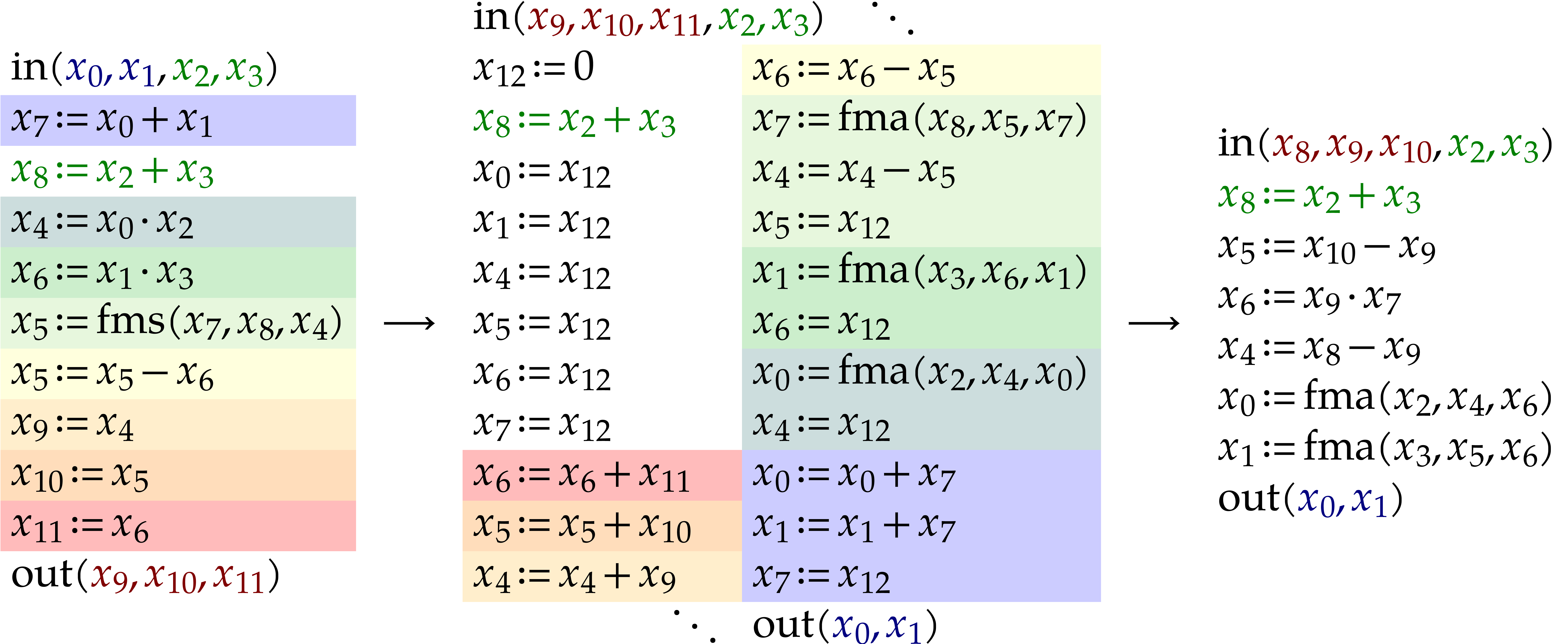
The left-hand SLP is a renumbered version of (5.2) to which we appended three instructions to copy the output (without this, the transposed SLP would override the input arguments). The middle SLP shows its raw unsimplified transposition. The background colors indicate the images of the individual instructions. For instance, the instruction

is equivalent to

which leads to the transposed code

. The instruction

is treated apart, because it only depends on the parameters

and not on the main input variables

: all instructions of this kind are extracted from the input SLP and prepended as is to the transposed SLP. For the transposition itself, the parameters

and variables like

are considered as constants. The right-hand SLP shows the simplification of the raw transposed SLP. We both applied usual simplification as in section 4.4 and an optimization that combines multiplications and additions into FMA instructions.

5.4.Homogenization

Consider a rational map

. Its homogenization is the rational map

such that

is homogeneous with

for

. The homogenization of an SLP can be constructed using a single linear pass, during which we keep track of the degrees of all intermediate results that were “computed” so far. The algorithm is best illustrated on an example:

The left-hand side shows the input SLP and the right-hand side its homogenization. We also indicate the degrees of all intermediate results. During additions, subtractions, and FMAs, we multiply with appropriate powers of

to keep things homogeneous. We also maintain a table of powers of

that were computed so far, in order to avoid needless recomputations.

This procedure actually extends to other operations, as long as the notion of degree extends in a reasonable way. For instance, for the operations

, and

, we may take

, and

5.5.SLP algebras

Let

be a fixed signature and let

be domains. We say that

is a domain over

if we have a function

in order to reinterpret elements in

as elements in

. Mathemagix comes with various fundamental template types that allow us to construct domains over

, like the domain

from section 5.1 or the domain

from section 5.2. As we saw in section 2.3, the Jil library uses an abstract data type domain and also provides constructors for many basic domains

over

Now consider the case when elements of

are represented as vectors in

and that

is implemented as an SLP

. Assume also that every operation

is implemented on

as an SLP

, where inputs

are represented as

. Then we call

an SLP algebra and call

its dimension over

. The recording technique from section 3 yields a convenient way to turn any domain

over

into an SLP algebra: we obtain

and every

by recording

and

over

. Conversely,

and

can be obtained from

and

through evaluation.

Remark 5.2. The examples of

and

from sections 5.1 and 5.2 are indeed

-algebras in the mathematical sense. In general, the signature

typically contains the algebra operations, but we do not insist on

to verify all mathematical axioms of an

-algebra.

Let

be a domain over

, whose elements are represented as vectors in

. Given an SLP

over

, we may naturally execute

over

. Using the recording technique from section 3, we may then obtain a new SLP, which we call the reinterpretation of

as an SLP over

. Similarly, since every operation in

can be applied over both

and

, and constants in

can be lifted to a constant in

, any SLP

over

can be evaluated over

. Recording the trace of such an evaluation, we obtain a new SLP that we call the lift of

. Note that this is still an SLP over

is actually an SLP algebra over

, then SLPs can be reinterpreted or lifted more efficiently using

and the

, while bypassing the recording technique. In sections 5.1 and 5.2, this is what we did in an ad hoc way for vectorization and forward differentiation. But something similar can be done to lift SLPs to general SLP algebras

. Given an input SLP

, we first renumber all data fields in

and the

such that they carry numbers

and such that each operations acts on separate data fields (some optimizations are actually possible here, but this is not crucial for the general idea). Essentially, it then suffices to replace every instruction

in the input SLP by

, while substituting

for the input arguments and

for the output arguments. The constant fields are lifted using

However, additional adjustments need to be made for instructions that involve aliasing. For instance, assume that

is the algebra of complex numbers over

, where

is implemented using the right-hand SLP from (2.3). Assume that

are variables that get lifted into

. Then the instruction

would a priori be lifted into

which is incorrect due to the aliasing. We thus have to do some additional renaming and/or copying in order to restore the correctness. In our example, it suffices to replace (5.3) by

where

are separate scratch variables. This corresponds to replacing our SLP (2.3) for complex multiplication by the following one in presence of aliasing:

In a similar way as at the end of sections 4.5 and 4.7, we should also avoid putting too much register pressure on the scratch variables

. This can be done by circulating the scratch variables among

possibilities, as usual.

Note that it can be detected automatically whether an SLP like the right-hand of (2.3) needs to be corrected when some of the arguments are aliased. Moreover, the appropriate correction may depend on the precise arguments that are aliased. For instance, consider the following implementation of complex FMAs:

A similar correction as in (5.4) is needed when lifting

, but no correction is needed when lifting

. In the Jil library, we dynamically construct and maintain a table of corrections for each kind of aliasing.

An interesting direction for future research would be to automatically combine certain instructions and lift them jointly. This would allow for heavier optimizations of the “joint lift” of the combined instructions. For instance, assume that we wish to lift an SLP that repeatedly contains the following pattern:

where

are pairwise distinct. We may view this pair of instructions as a joint instruction

This instruction might be lifted as a single instruction over the SIMD type

. As highlighted in section 5.1, this typically yields a “joint lift” of better quality than sequentially lifting the instructions

and

. More generally, we expect rescheduling as in section 4.6 to be an interesting optimization on this kind of joined lifts.

5.6.Ball arithmetic

Ball arithmetic [60, 76] is a variant of interval arithmetic [91, 92, 102]. Given a numerical algorithm and an input, the aim is to automatically compute a rigorous bound for the error of the output. In our case, the algorithm will be given by an SLP.

The idea behind ball arithmetic is to systematically replace approximate numbers by balls that enclose the true mathematical values. According to this semantics, a ball lift of an operation

(which we will still denote by

) takes balls

as inputs and produces a ball

that satisfies the inclusion property:

In order to construct such ball lifts, we also have to take into account rounding errors, when working with finite precision.

For instance, let

be the set of standard IEEE-754 double precision floating point numbers. Given an operation

on real numbers, let

denote its correctly rounded variant on

. Given

and

, let

be the ball with center

and radius

. Then the standard arithmetic operations can be lifted as follows:

Other operations can be lifted similarly. Taking

, this allows us to implement

as an SLP algebra (note that

is not an algebra in the mathematical sense though: remind Remark 5.2). Lifting an SLP

over

, we obtain a new SLP

that computes the usual numerical evaluation of

, together with a rigorous error bound for the obtained approximate value.

The SLP

obtained through direct lifting has the disadvantage that a lot of time is spent on evaluations of

, i.e. on bounding rounding errors. It turns out that this can entirely be avoided by slightly increasing the radii of input balls. The precise amount of inflation can be computed as a function of the input SLP

: see [70, Theorem 5] for a formula. The fact our program

is an SLP allows us to do this computation statically, i.e. while building the output program

and not merely while executing it. This is not possible for general purpose programs

that may involve loops of unpredictable lengths or recursions of unpredictable depths.

Ball arithmetic can be generalized [59, 70] to balls with centers in more general algebras such as the complexification

. However, the formula

for the absolute value of a complex number

involves a square root, which is fairly expensive to compute. In [70], we proposed to compute these absolute values using the formula

whenever we need to lift a product

. In Justinline we implemented this as an ad hoc optimization. An alternative approach is to implement a separate SLP algebra for “complex balls with absolute values”. Such balls are of the form

, where

, and

. Ignoring rounding errors, we may implement the standard arithmetic operations as follows:

After lifting an SLP over

, we may again “forget” about the absolute values and project the output down to

. Removing all dead code from the resulting SLP (see section 4.2), we essentially obtain the same SLP as using the ad hoc implementation from Justinline. The advantage of the alternative approach is that its correctness is more straightforward. It also directly extends to other operations such as division or square root. On the downside, it is a bit slower to first insert instructions that compute unneeded absolute values, only to remove them later during the dead code elimination.

5.7.Modular arithmetic

There are several ways to implement modular arithmetic in

when

. We refer to [73] for a survey of efficient methods that can benefit from SIMD acceleration. In this section, we will use a variant of modular arithmetic that is based on machine double precision arithmetic, but the material can easily be adapted to other variants.

As in the previous subsection, we assume that our hardware implements the IEEE-754 standard for floating point arithmetic and we use rounding to the nearest. Recall that integers in

can be represented exactly in

. We assume that our modulus is odd with

and also assume that

has been precomputed.

We represent a normalized residue modulo

as an integer in

between

and

. The normal form

of an integer

can be computed efficiently using the

operation as follows:

Here

stands for the closest integer near

. Abbreviating this code by

, this naturally leads to the following algorithms to compute the modular sum, difference, and product

and

Let

be the SLP algebra over

, where the arithmetic operations are implemented in this way.

In the algorithms (5.6), we note that the bulk of the computation time is spent on modular reductions. A common technique to avoid reductions is to delay them as much as possible [28, 29, 54, 18, 105]. This can be achieved by switching to a non-normalized or redundant representation of residues modulo

by integers in the range

. In the above algorithms (5.6), we may then suppress the final reduction

, whenever we are able to guarantee that

. In the contrary case, we will say that the operation overflows for the corresponding inputs

and

Let

be the SLP algebra that corresponds to the above kind of non-normalized modular arithmetic:

We also extend

with an operation “

” that is implemented as the identity operation by default and as modular reduction (5.5) on

. Now consider an SLP

over

with inputs

. In absence of overflows, its execution over

produces the same output modulo

as its execution over

. The correctness of the optimized execution over

can be restored in presence of overflows by inserting a reduction after every instruction that may cause an overflow.

How to determine and correct the instructions that may cause overflows? In [72, section 4.1], we described a simple greedy algorithm for doing this. Roughly speaking, we start with the bounds

for the absolute values of our inputs. Using a linear pass through our SLP, we next compute bounds for the results of every instruction: for additions and subtractions

, we have

; for multiplications

, we have

. Whenever the bound for

exceeds

, we insert the instruction

, and replace the bound by

. Optionally, we also insert instructions to reduce all output values at the end of the SLP.

The redundant representation for the residues modulo

allows for some additional optimizations. For instance, we may use the following algorithm for the fused operation

modulo

Although this implementation is not faster than the default implementation (a modular multiplication followed by a modular addition), it yields a better bound for the result: we obtain

instead of

. This optimization may therefore help to lower the number of reductions that need to be inserted in order to counter potential overflows. Note that this subtle improvement is hard to find automatically and also requires us to include the “fma” operation into

(remember the discussion in section 2.2).

Let us finally investigate the role of the modulus

. In a typical C++ implementation, this is either a template parameter (in which case a recompilation is necessary in order to use a new

) or we pass it as an additional function argument (in which case, we cannot exploit special properties of

at compile time). In our SLP setting, we dynamically generate specific code for any required modulus

, while relying on the ability to “efficiently generate disposable machine code”. The specific value of

was for instance used during the above bound computations. Certain simplifications may also exploit it, e.g. if a constant happens to be a multiple of

plus zero, one, or minus one.

We may sometimes prefer to create SLPs for generic moduli

. This remains possible, e.g. by treating

as an input variable when recording. Of course, special restrictions will apply in this case, since it is no longer possible to do static optimizations that take into account the specific value of

. For instance, it is necessary to tweak the above procedure to counter overflows: the bound

for multiplication must be replaced by

, where

is a fixed upper bound for the target moduli

5.8.Extended precision arithmetic

There are various ways to conduct numerical computations with a precision that exceeds the hardware precision. Popular libraries like Gmp and Mpfr [49, 35] represent unsigned multiple precision integers as

, where

are machine integers that are often called limbs. The efficient implementation of basic arithmetic then relies on hardware support for carry handling. For instance, the addition of two numbers of

limbs is implemented as follows on traditional hardware:

Unfortunately, this code is not an SLP according to our definition, because the semantics of the carry handling is implicit: if this were an SLP, then the three additions would be independent, so permuting them in any order would yield an equivalent SLP. Various approaches to reconcile carry handling with our SLP framework will be presented in a forthcoming paper. Of course, one may also directly generate assembly code for programs like (5.8), as a function of the desired extended precision [2].

Another disadvantage of the reliance on carries is that SIMD units do not always support them. For instance, neither AVX2, AVX512, nor Neon provide a vector version of “add with carry”. Nvidia GPUs do support carries, but only through Ptx. One remedy to this problem is to use a redundant representation of multiple precision integers, like

with

, and reserve the

highest bits of

for carry handling. This representation is particularly interesting on recent Intel and Amd processors with support for the IFMA instructions: the unnormalized SIMD multiplication of two such integers can then be done in only

cycles [50, 31].

On CPUs and GPUs without efficient carry handling or IFMA instructions, one may rely on floating point arithmetic for efficient SIMD implementations of extended precision arithmetic. This is particularly interesting if the hardware favors floating point over integer arithmetic. In [69], we showed how to efficiently implement medium precision fixed point arithmetic in this way. Fixed point numbers can be represented redundantly as

, with

, where

is a small number that corresponds to the number of “carry bits” (one typically has

). The unnormalized SIMD multiplication of two such numbers takes approximately

cycles. The techniques from [69] can be adapted to multiple precision integer arithmetic.

The above fixed point numbers form an SLP algebra, when

and

are fixed. As in the case of modular arithmetic, there is an operation “

” to put numbers in an almost normal form with

for

. Using a similar greedy algorithm as in the previous subsection, we may detect potential overflows and deal with them by inserting appropriate reductions. In the case of fixed point arithmetic, this gives rise to a trade-off: if we increase

by one, then we may lower the number of reductions, but also lose

bits of precision.

We may next develop floating point arithmetic on top of integer or fixed point arithmetic by managing all exponents ourselves. This approach is for instance used in Gmp and Mpfr, but it is less suited for SIMD parallelization. Shift operations on mantissas are indeed non-trivial to implement in an SIMD fashion: see [64] for some experiments in that direction. For the evaluation of an SLP on a bounded region, an alternative idea is to statically compute bounds for all exponents encountered during the computation. If we allow mantissas to be non-normalized (i.e. the leading bits could be zero), then we may use these bounds (possibly rounded up to a multiple of the bit-size of limbs) as our exponents and greatly reduce the cost of shifting.

Another way to extend the precision of floating point arithmetic is to use compensated algorithms such as 2Sum [89]. In that case, a floating point number with

-fold precision is represented as

, where

are hardware floating point numbers that do not overlap (for double precision, this typically means that

for

). Algorithms for basic arithmetic operations in doubled precision (

) go back to [25]. We refer to [99, 12, 78] for generalizations to higher precisions. For a fixed value of

, this type of arithmetic again gives rise to an SLP algebra. Since the representation is normalized, no special reductions are needed to counter carry overflows. (However, additional efforts are required in order to fully treat floating point errors, overflows, and underflows.) Unfortunately, the overhead of the compensated algorithms approach tends to increase rapidly as a function of

, which limits its practical usefulness to the case when

6.Applications

In this section, we discuss several applications for which we started using or plan to use our SLP libraries. We will highlight the added value of the SLP framework, and also investigate limitations and ideas to work around them. The list of selected applications is by no means exhaustive, but it will allow us to cover a variety of issues that are relevant for the development of SLP libraries.

6.1.Homotopy continuation

Numerical homotopy continuation [4, 104] is the archetype application of SLPs. Assume that we wish to solve a polynomial system

that is easy to solve. This typically means that both systems have the same number of solutions and the same total degrees:

. Now consider the following system that depends a “time” parameter

For

and

this system reduces to (6.1) and (6.2), respectively. The idea is then to follow the solutions of (6.2) from

. This can be achieved using various “path tracking” algorithms. The most straightforward method uses Euler–Newton iterations: given an approximate solution

at time

, we get an approximate solution

at time

using

This formula can be used both as a predictor (with

) and as a corrector (with

). One typically alternates prediction and correction steps. In order to control the step-size

, one uses a predicate for deciding whether a step needs to be accepted: in case of acceptance, we increase the step-size (say

); otherwise, we decrease it (say

). A simple predicate that one may use is

but other predicates may be suitable for certain systems. The quality of the first order approximation (6.3) can also be improved: if we have approximations

and

of the solution

at two successive times

, together with approximations

and

of the gradient

, then we may fit

using a polynomial of degree

, and use that to obtain a higher order approximation at a new time

In the context of this paper, it is convenient to regard our systems as zeros of polynomial mappings

, and

that are given through SLPs. Using automatic differentiation, we may then construct SLPs for

and

. We may also record linear algebra routines for matrix multiplication, inversion, and norm computation. This enables us to construct SLPs for steppers (6.3) and verifiers (6.4).

The SLP framework has several advantages here. If our polynomials are sparse, then evaluation in the SLP representation may be significantly faster. Moreover, the sparsity is conserved by automatic differentiation. Even in the dense representation, the monomials are shared subexpressions between

, so the evaluation of

is typically faster than the separate evaluation of

. Furthermore, we generate machine code for the evaluation, which is faster then using a loop over the terms of an expanded representation of

Full fledged SLP libraries also provide a lot of flexibility concerning the domain

. Usually, we take

to be the domain of machine complex floating point numbers at double precision. But we may easily lift our SLPs to extended precision, as we saw in section 5.8. The techniques from section 5.6 also allow us to efficiently evaluate SLPs over balls and then use this to construct certified path trackers [83, 62]. Generating machine code for evaluating a given SLP over

is fast, provided that we have efficient implementations for the methods from sections 3, 4 and 5.5. In the SLP framework such codelets can thus be constructed on-the-fly whenever needed for the resolution of our specific input system. Similarly, if a system has multiple solutions, then automatic differentiation can be used to “deflate” it on-the-fly into a system which turns these solutions into isolated ones.

Numerical homotopy methods lend themselves very well to parallelization, since every separate path can be tracked using a different thread. SIMD acceleration of width

may also be used to simultaneously track

paths using a single thread. However, the required number of steps may differ from one path to another, so an ad hoc mechanism is needed to detect complete paths and to feed the corresponding threads (or SIMD lanes) with new paths. The strict SLP framework is slightly insufficient for implementing such a mechanism. A minima, when generating machine code for our SLP, we wish to be able to surround it by a loop that allows for multiple executions until some condition is met. As briefly discussed in section 4.9, this kind of control sugar is a welcome extension of the framework from this paper.

6.2.Discrete Fourier transforms

Another major application of SLP libraries is the automatic generation of codelets for discrete Fourier transforms (DFTs) and variants.

The codelet approach was pioneered in FFTW3 [37, 38] and later applied in other implementations [100, 72]. Given any desired order, the idea is to automatically generate a dedicated and highly optimized codelet to perform DFTs of this order. For small orders, the appropriate codelet is typically unrolled as an SLP and pre-compiled into the library. For larger orders, the idea is to decompose the transform into DFTs of smaller orders using classical techniques due to Good, Cooley–Tukey, Rader, etc. There are often many competing algorithms to compute a DFT, in which case we automatically compare running times and select the best strategy for the target length. This tuning phase may be expensive, but the best strategies can be cached.

In order to achieve really high performance, it is actually profitable to unroll DFTs up till “not so small” orders like

. When pre-compiling all these “not so small” DFTs into the library, this may considerably blow up its size. This is all the more true if one also wishes to include variants of DFTs such as the truncated Fourier transform [56, 58, 84]. In the SLP framework, one may efficiently build and compile these codelets on-the-fly, while preserving or even improving the efficiency at execution time.

The SLP approach is also more versatile, because it allows us to dynamically choose our ground ring

. Traditional DFTs over

may therefore be generated on-the-fly for various working precisions. But one may also generate number theoretic transforms over

for various prime numbers

[97], and Nussbaumer polynomial transforms [94] over

for various degrees

. In addition, we may apply algebraic optimization techniques from section 5, while exploiting particular mathematical properties of the ground ring

. This idea has been applied successfully in [69, 66, 72] for DFTs in medium precision and number theoretic transforms over

, and

for so-called smooth FFT primes

A few technical issues need to be addressed though in order to use an SLP library for this application. First of all, the design of DFTs of large orders heavily relies on tensor products [100]: given an SLP

that computes a DFT (or another linear map) of order

, we often need highly optimized code for

and

. If

is small, then we simply generate SLPs for these tensor products. However, if

and

are both “not so small”, then it is best to automatically put the code of

inside a loop of length

. This is another instance where control sugar is useful (see also sections 4.9 and 6.1). Moreover, we may wish to pass

as a parameter to the functions

and

Another issue is to find the best strategy for computing a particular DFT. Our SLP library must therefore contain support for benchmarking competing strategies on-the-fly and selecting the best ones. Such a mechanism can be expensive, so this should be complemented by a caching system that remembers the best strategies. This is a non-trivial problem that we have not yet addressed in our present implementations. For instance, for DFTs of a fixed length over

, should we use the same strategy for different values of

? We might also attempt to cleverly bench a reduced number of DFTs and try to build a model that can predict the running time of other DFTs.

6.3.Relaxed power series and differential equations

Consider the multiplication

of two formal power series

. From an algorithmic perspective, we may deal with the infinite nature of power series in several ways. One idea is to work at a finite truncation order: given

and

, we then wish to compute

. Another approach [57], the relaxed (or online) one, is to regard

and

as streams of coefficients and to insist that

needs to be output as soon as

and

are known. The naive way to compute the product

in a relaxed manner is to directly use (6.5). At order three, this yields

In fact, Karatsuba's algorithm is essentially relaxed [57], modulo reordering the instructions in an appropriate way. However, this reordering is non-trivial to program and the appropriate control structures induce a significant overhead. Our SLP framework has a big advantage here, since, no matter how complex these control structures are, the overhead vanishes when recording the multiplication.

Example 6.1. Relaxed multiplication has the property that the coefficients

and

of the inputs are allowed to depend on earlier coefficients

of the output. This yields a convenient way to solve power series equations. For instance, the inverse

of a power series of the form

satisfies the equation

Now assume that we compute

using the formula

and Karatsuba's algorithm. When recording the trace of an expansion at order

, we obtain the following SLP, after simplification:

Trading one multiplication against several additions and subtractions may not seem worth the effort, except maybe for larger orders. However, when lifting the SLP to a domain like

from section 5.7, multiplications may be far more expensive than additions and subtractions. Even for small orders, the relaxed approach may then lead to significant savings.

, then the relaxed approach can in particular be used in order to solve a system of ordinary differential equations (ODEs) of the form

after which one may check that the coefficients

only depend on earlier coefficients when evaluating the right-hand sides.

For any given truncation order

, we may record the resolution process as an SLP. The power series solution naturally gives rise to a “stepper” for the numerical integration of the system. However, the size of the SLP increases with

: the factor is

for the naive method,

for Karatsuba's method, and

for large

(see [57, 63] for asymptotically fast methods). It is an interesting problem to rewrite this SLP as multiple applications of a few SLPs of significantly smaller sizes (about

SLPs of the size of the original SLP might do, by associating one type of SLP to each size of squares in [57, Figure 3] and doing the required transforms separately). This also raises the practical challenge of generating SLPs that call other SLPs: another example of control sugar.

Traditional Runge-Kutta methods for the numerical integration of ODEs are also very suitable for the SLP framework. They have the advantage that they just require an SLP for the evaluation of the polynomials

. However, efficient Runge–Kutta schemes are only known up till order

: for larger orders, we need many evaluations, so Taylor series methods are currently more efficient.

6.4.Multiple precision arithmetic

In section 5.8 we already discussed the generation of SLPs for arithmetic operations with extended precision. The typical application that we had in mind there was to allow for SLPs over numerical domains with a fixed higher precision. In order to support integers and rational numbers as domains

, we also need to consider mixed precisions. The same holds when solving some equation over high precision floating point numbers using Newton's method: in this case, it is best to double the working precision at every iteration.

The most straightforward way to compute with mixed precisions is to use a similar interface as Gmp or Mpfr: the precision is either part of the data structure or passed as a parameter. Consider for instance the multiplication of two integers of

limbs. For small values of

, we may automatically generate a dedicated routine, similarly as in section 5.8. We may still do this for “not so small values” of

, in which case we may unroll Karatsuba's and Toom's more sophisticated multiplication algorithms [82, 106]. For larger

, we may recurse down to these base cases for which we generated dedicated implementations. For very high precisions, we may resort to FFT-multiplication [97], where the appropriate number theoretic transforms are automatically generated using the techniques from section 6.2. A similar strategy can be applied for the multiplication of two integers of different sizes in limbs.

It is a good question whether the general master routine for integer multiplication should also be generated automatically by the SLP library. It is not unreasonable to require that the implementation of such routines should be done in a separate higher level library. But it might also be interesting if the SLP library could automatically generate a full library like Gmp itself. However, this will require further control sugar, since most master routines for arithmetic operations will involve branching on the limb size, potentially using a lookup table. In fact, we may even build and cache the machine code for a certain size only when it is needed.

Another mixed precision scenario is the evaluation of an SLP over the integers

, where we have bounds for the input arguments. In that case, we can statically determine bounds for the results of all instructions and their sizes in limbs. We may next replace each instruction by a dedicated SLP for the corresponding number of limbs. Consider for instance the computation of the product

of integers

that all fit into one limb. This can efficiently be done using the technique of product trees: for

, we compute

using an SLP for

limb multiplication,

and

using an SLP for

limb multiplication, and

using an SLP for

limb multiplication.

A major shortcoming of existing multiple precision libraries like Gmp and Mpfr is that they do not fully exploit SIMD parallelism. In order to do so, one should start with an extension of the user interface, by providing vector versions of all basic routines. E.g., multiplying

integers at a time:

. This is not entirely convenient, because an SIMD routine for doing this requires all

to be of the same limb size and similarly for the

. But there exist many applications for which the sizes of integers are indeed predictable and uniform. The SLP framework naturally allows us to speed up such applications by generating SIMD versions of operations on integers.

6.5.Geometric resolution

Last but not least, we hope that our new SLP libraries will be useful in order to speed up polynomial system solving using the method of geometric resolution. This method can be thought of as a purely algebraic counterpart of homotopy continuation from section 6.1, although the technical details are very different. It was first developed by Joos Heintz and his collaborators [43, 45, 41, 44] from a theoretical complexity standpoint. The second author and collaborators further improved the method and also implemented it [48, 85, 86, 30, 71].

The aim is again to solve a system of polynomial equations (6.1), but we now work over an effective field

instead of

. The solutions typically lie in an extension field

. A primitive representation

is therefore computed along with the solutions itself, where

us a monic irreducible polynomial. For sufficiently generic systems, the degree of

coincides with the number of solutions and all solutions can be represented simultaneously via a single point in

(each root of

giving rise to an actual solution).

Unlike numerical homotopy continuation, the geometric resolution method proceeds by an induction over the dimension. Assume that we have a solution of the

-dimensional system

over

, where

is a time parameter as in section 6.1. Expansions of order

will generically suffice. We next intersect the “solution curve”

of the system (6.7) with the hypersurface of zeros of

. It turns out that the resulting equation

can be solved using one big resultant computation. If

, then it is also profitable to first reduce the system modulo a small and suitable “machine” prime

, solve the resulting system over

, Hensel lift the solution to

, and finally obtain the desired solution using rational number reconstruction [40, section 5.10].

In order to implement this strategy efficiently, the following basic building blocks are particularly crucial: fast univariate polynomial arithmetic over

, fast arithmetic modulo

, efficient evaluations of SLPs over

and

, efficient algorithms for resultants and subresultants, and variants of these building blocks when working over

instead of

. Now univariate polynomial arithmetic over

is very similar to integer arithmetic. Using a similar approach as in the previous subsection, we may benefit from the SLP framework to automatically generate the required routines.

If the degree of

gets large, then multiplications in

are done using fast Fourier methods. When evaluating an SLP over

, a lot of the required DFTs can often be shared, which significantly reduces the cost. Similarly, reductions modulo

can often be postponed to the end. For instance, the

matrix product (3.4) can be lifted from

as follows: we first convert the input arguments

into the FFT representation using DFTs, then perform the

matrix multiplication while using the FFT representation, next convert the result back into the usual polynomial representation, and finally reduce modulo

In order to implement such optimizations within our SLP framework, it is convenient to extend the signature

with converters between the polynomial and FFT representations and with operations on the FFT representations. This will allow us to lift (3.4) as follows from

Here elements of

are represented redundantly by polynomials of degree

, where

. The operation “reduce” computes the remainder of the division by

. The input arguments are assumed to be reduced. The map

computes a discrete Fourier transform of length

(assuming that

has a

-th primitive root of unity), where

. This map is

-linear and we have

for polynomials

. We noted

and

for the vector lifts of

and

In fact, the cost of the reductions (which also require FFT multiplications) can be further reduced by switching to a polynomial analogue [88] of the Montgomery representation [90] for elements of

. One may also consider Fourier representations of larger sizes

, ...: this increases the cost of individual transforms, but may dramatically reduce the number of transforms that need to be done. We plan to further work out the details of these ideas in a forthcoming paper.

7.Benchmarks

As stated in the introduction, our previous papers [70, 66] internally rely on the Justinline library. In particular, the benchmarks in these papers provide early evidence that the SLP approach can greatly boost performance. In this section, we mainly report on preliminary timings for the Jil library, for an experimental

-version that has just been released [1].

7.1.Test platforms

7.2.Basic operations on SLPs

Our first benchmark concerns the computation of determinants of

matrices. We consider two types of input SLPs for computing this determinant:

The Tables 7.1, 7.2, and 7.3 have been subdivided into two main left-hand and right-hand parts which correspond to the naive and simplified SLPs, respectively. The first “len” column shows the number of instructions of the input SLP. Each other column reports the timing of a specific operation on the input SLP in cycles per instruction:

Tables 7.1 , 7.2 , and 7.3 report timings for our three test platforms M3 , Xeon , and Ryzen , respectively.

One major observation concerning these tables is that all operations on SLPs require between 100 and 1000 cycles per instruction, approximately. The older Intel Xeon processor is a bit slower than the more recent AMD Ryzen and Apple M3 processors. Machine code generation is significantly faster for the M3, which is due to the simpler instruction encoding for this ARM RISC processor.

For small values of

, the timings involve a large overhead. This overhead tends to disappear for SLPs with more than 100 instructions. The timings remain relatively stable in the midrange, for SLPs of lengths between 100 and 100000. Very large SLPs cause cache problems and we observe a significant overhead for such SLPs.

For input SLPs of midrange lengths, we note that instructions tend to execute in less than one cycle. This is due to out of order execution by multiple execution units, which is particularly well done on M3 processors. We also note that all cycle times are reported with respect to the base clock speed.

We recall that domain for all timings in Tables 7.1, 7.2, and 7.3 is the scalar domain

of double precision floating point numbers. For many applications, it is possible to work over the SIMD domain

for some

, in which case multiple executions are accelerated by an approximately factor of

with respect to

. This allows the Xeon and Ryzen platforms (on which

) to make up for the smaller number of execution units with respect to the M3 platform (on which

). See [72, section 5.1] for more details on this point and further benchmarks.

Let us finally examine the kind of code that is generated by our SLP simplifier. In Figure 7.1 , we show the simplified SLP for computing a

determinant, as well as the corresponding machine code on X86 platforms. We observe that the code makes efficient use of fused multiply add instructions. The generated machine code also tends to exploit the indirect addressing mode for arithmetic instructions whose arguments are only required once. For small values of

, the simplified SLPs are quite competitive with Gaussian elimination. They have the advantage that they require no divisions and no conditional code to find appropriate pivots.

7.3.Homotopy continuation

One major motivation for our work on SLP libraries is the development of a fast tool for numerical homotopy continuation at double precision.

We did a first prototype implementation in Mathemagix, based on the Justinline library. This experimental code uses Mathemagix in a complex way and is not suitable for public distribution. The SIMD width is limited to 256 bits (four double precision numbers), but we implemented a second order predictor-corrector scheme, with carefully fine-tuned parameters.

We recently started a C++ reimplementation inside the Jil library. This code supports the full 512 bit SIMD width (eight double precision numbers), but, so far, we only implemented the most straightforward first order stepper (6.3).

In Table 7.4 , we reported timings for the classical Katsura benchmark. We also consider a few dense random systems Posso of dimension

and total degree

. The first “sols” column shows the total number of solutions. The columns labeled by “jit” indicate the time spent on building the machine code. The columns labeled by “exe ” show the actual time that was needed to solve the system using

threads.

The main benefit of switching to our lower level implementation in Jil is a dramatic speed-up (between 10 and 100, approximately) for the building time of machine code: the major problem for our Mathemagix implementation is indeed that the building time exceeds the parallel execution time for systems with up till around 100000 solutions. Nonetheless, despite the halved SIMD width, the running times for the solver itself are very competitive. This shows that there is still room for algorithmic improvements in our present Jil implementation.

More extensive benchmarking reveals that the performance scales well with the number of threads and the SIMD width on our test platforms. The last two columns of Table 7.4 show that this even holds when passing from 6 to 12 threads on the M3 processor: for the particular application of path tracking, efficiency cores perform almost as well as performance cores. Curiously, on the Xeon platform, our Jil implementation suffers from a large overhead for systems with less than

solutions; we are still investigating the reason for this.

One major objective of the Jil library is to also support GPUs besides CPUs. Work in this direction has only started recently with the implementation of a rudimentary OpenCL interface. In Table 7.5 , we report some first timings. We note that the overhead of the OpenCL compiler is very large, typically between 100 and 1000. As a consequence, the building time dominates the cost except for very large systems. We also observed disappointing execution times, despite the “embarrassingly parallel” nature of our application. This is partly due to the fact that we work with double instead of single precision. But we are still far from the theoretical peak performance, even for double precision. OpenCL also seems to be a suboptimal choice. On NVidia cards, a native Cuda or Ptx interface would probably be more efficient.

Bibliography

[1]: A. Ahlbäck, J. van der Hoeven, and G. Lecerf. https://sourcesup.renater.fr/projects/jil, 2025.
[2]: A. Ahlbäck and F. Johansson. Fast basecases for arbitrary-size multiplication. In 2025 IEEE 32nd Symposium on Computer Arithmetic (ARITH), pages 53–60. 2025.
[3]: A. V. Aho, M. S. Lam, R. Sethi, and J. D. Ullman. Compilers principles, techniques & tools. Pearson Education, 2nd edition, 2007.
[4]: Georg, K. Allgower, E. L. Numerical Continuation Methods. Springer-Verlag, 1990.
[5]: ANSI/IEEE. IEEE standard for binary floating-point arithmetic. Technical Report, ANSI/IEEE, New York, 2008. ANSI-IEEE Standard 754-2008. Revision of IEEE 754-1985, approved on June 12, 2008 by IEEE Standards Board.
[6]: ARM corporation. Fast models user guide. https://developer.arm.com/documentation/100965/latest. Version 11.29.
[7]: M. Aschenbrenner, L. van den Dries, and J. van der Hoeven. Asymptotic Differential Algebra and Model Theory of Transseries. Number 195 in Annals of Mathematics studies. Princeton University Press, 2017.
[8]: AsmJit: low-latency machine code generation. https://github.com/asmjit/asmjit.
[9]: Autodiff: automatic differentiation in C++ couldn't be simpler. https://autodiff.github.io.
[10]: Torch.autograd: automatic differentiation package in pytorch. https://docs.pytorch.org/docs/stable/autograd.html.
[11]: Awesome-JIT. https://github.com/wdv4758h/awesome-jit. Ressources for JIT compilation.
[12]: D. H. Bailey, Y. Hida, and X. S. Li. Algorithms for quad-double precision floating point arithmetic. In 15th IEEE Symposium on Computer Arithmetic, pages 155–162. IEEE, 2001.
[13]: H. G. Baker. Computing A*B (mod N) efficiently in ANSI C. SIGPLAN Not., 27(1):95–98, 1992.
[14]: W. Baur and V. Strassen. The complexity of partial derivatives. Theor. Comput. Sci., 22:317–330, 1983.
[15]: Blas (basic linear algebra subprograms). https://netlib.org/blas/.
[16]: J. L. Bordewijk. Inter-reciprocity applied to electrical networks. Applied Scientific Research B: Electrophysics, Acoustics, Optics, Mathematical Methods, 6:1–74, 1956.
[17]: A. Bostan, G. Lecerf, and É. Schost. Tellegen's principle into practice. In Proceedings of the 2003 International Symposium on Symbolic and Algebraic Computation, ISSAC '03, pages 37–44. New York, NY, USA, 2003. ACM Press.
[18]: J. Bradbury, N. Drucker, and M. Hillenbrand. NTT software optimization using an extended Harvey butterfly. Cryptology ePrint Archive, Paper 2021/1396, 2021. https://eprint.iacr.org/2021/1396.
[19]: P. Briggs, K. D. Cooper, and L. Torczon. Rematerialization. In Proceedings of the ACM SIGPLAN 1992 Conference on Programming Language Design and Implementation, PLDI '92, pages 311–321. New York, NY, USA, 1992. ACM.
[20]: N. Bruno, J. Heintz, G. Matera, and R. Wachenchauzer. Functional programming concepts and straight-line programs in computer algebra. Math. Comput. Simulation, 60(6):423–473, 2002.
[21]: P. Bürgisser, M. Clausen, and M. A. Shokrollahi. Algebraic complexity theory. Springer-Verlag, Berlin, 1997.
[22]: B. Castaño, J. Heintz, J. Llovet, and R. Martìnez. On the data structure straight-line program and its implementation in symbolic computation. Math. Comput. Simulation, 51(5):497–528, 2000.
[23]: G. J. Chaitin. Register allocation & spilling via graph coloring. ACM Sigplan Notices, 17(6):98–101, 1982.
[24]: G. J. Chaitin, M. A. Auslander, A. K. Chandra, J. Cocke, M. E. Hopkins, and P. W. Markstein. Register allocation via coloring. J. Comput. Lang., 6(1):47–57, 1981.
[25]: T. J. Dekker. A floating-point technique for extending the available precision. Numer. Math., 18(3):224–242, 1971.
[26]: A. Díaz and E. Kaltofen. FoxBox: a system for manipulating symbolic objects in black box representation. In Proceedings of the 1998 International Symposium on Symbolic and Algebraic Computation, ISSAC '98, pages 30–37. New York, NY, USA, 1998. ACM.
[27]: J.-G. Dumas, T. Gautier, M. Giesbrecht, P. Giorgi, B. Hovinen, E. Kaltofen, B. D. Saunders, W. J. Turner, and G. Villard. LinBox: a generic library for exact linear algebra. In A. M. Cohen, X. S. Gao, and N. Takayama, editors, Proceedings of the 2002 International Congress of Mathematical Software, Beijing, China, pages 40–50. World Scientific, 2002. https://linalg.org.
[28]: J.-G. Dumas, P. Giorgi, and C. Pernet. FFPACK: finite field linear algebra package. In J. Schicho, editor, Proceedings of the 2004 International Symposium on Symbolic and Algebraic Computation, ISSAC '04, pages 119–126. New York, NY, USA, 2004. ACM.
[29]: J.-G. Dumas, P. Giorgi, and C. Pernet. Dense linear algebra over word-size prime fields: the FFLAS and FFPACK packages. ACM Trans. Math. Softw., 35(3):19–1, 2008.
[30]: C. Durvye and G. Lecerf. A concise proof of the Kronecker polynomial system solver from scratch. Expo. Math., 26(2):101–139, 2008.
[31]: T. Edamatsu and D. Takahashi. Accelerating large integer multiplication using intel AVX-512IFMA. In Algorithms and Architectures for Parallel Processing: 19th International Conference, ICA3PP 2019, Melbourne, Australia, pages 60–74. Springer-Verlag, 2019.
[32]: Ch. M. Fiduccia. On the algebraic complexity of matrix multiplication. PhD thesis, Brown University, 1973.
[33]: N. Fitchas, M. Giusti, and F. Smietanski. Sur la complexité du théorème des zéros. In M. Florenzano and J. Guddat, editors, Approximation and optimization in the Caribbean, II (Havana, 1993), volume 8 of Approx. Optim., pages 274–329. Frankfurt am Main, 1995. Lang.
[34]: A. Fog. Software optimization resources. https://www.agner.org/optimize.
[35]: L. Fousse, G. Hanrot, V. Lefèvre, P. Pélissier, and P. Zimmermann. MPFR: a multiple-precision binary floating-point library with correct rounding. ACM Trans. Math. Software, 33(2), 2007. Software available at https://www.mpfr.org.
[36]: T. S. Freeman, G. M. Imirzian, E. Kaltofen, and Y. Lakshman. DAGWOOD: a system for manipulating polynomials given by straight-line programs. ACM Trans. Math. Software, 14:218–240, 1988.
[37]: M. Frigo. A fast Fourier transform compiler. In Proc. 1999 ACM SIGPLAN Conf. on Programming Language Design and Implementation, volume 34, pages 169–180. ACM, May 1999.
[38]: M. Frigo and S. G. Johnson. The design and implementation of FFTW3. Proc. IEEE, 93(2):216–231, 2005.
[39]: M. Frigo, C. E. Leiserson, H. Prokop, and S. Ramachandran. Cache-oblivious algorithms. In 40th Annual Symposium on Foundations of Computer Science, pages 285–297. IEEE, 1999.
[40]: J. von zur Gathen and J. Gerhard. Modern Computer Algebra. Cambridge University Press, 3rd edition, 2013.
[41]: M. Giusti, K. Hägele, J. Heintz, J. L. Montaña, J. E. Morais, and L. M. Pardo. Lower bounds for diophantine approximations. J. Pure Appl. Algebra, 117/118:277–317, 1997.
[42]: M. Giusti, K. Hägele, G. Lecerf, J. Marchand, and B. Salvy. The projective Noether Maple package: computing the dimension of a projective variety. J. Symbolic Comput., 30(3):291–307, 2000.
[43]: M. Giusti and J. Heintz. La détermination des points isolés et de la dimension d'une variété algébrique peut se faire en temps polynomial. In D. Eisenbud and L. Robbiano, editors, Computational algebraic geometry and commutative algebra (Cortona, 1991), Sympos. Math., XXXIV, pages 216–256. Cambridge Univ. Press, 1993.
[44]: M. Giusti, J. Heintz, J. E. Morais, J. Morgenstern, and L. M. Pardo. Straight-line programs in geometric elimination theory. J. Pure Appl. Algebra, 124(1-3):101–146, 1998.
[45]: M. Giusti, J. Heintz, J. E. Morais, and L. M. Pardo. When polynomial equation systems can be “solved” fast? In G. Cohen, M. Giusti, and T. Mora, editors, Applied Algebra, Algebraic Algorithms and Error-Correcting Codes. AAECC 1995, volume 948 of Lect. Notes Comput. Sci., pages 205–231. Springer-Verlag, 1995.
[46]: M. Giusti, J. Heintz, J. E. Morais, and L. M. Pardo. Le rôle des structures de données dans les problèmes d'élimination. C. R. Acad. Sci. Paris Sér. I Math., 325(11):1223–1228, 1997.
[47]: M. Giusti, J. Heintz, and J. Sabia. On the efficiency of effective Nullstellensätze. Comput. Complexity, 3(1):56–95, 1993.
[48]: M. Giusti, G. Lecerf, and B. Salvy. A Gröbner free alternative for polynomial system solving. J. Complexity, 17(1):154–211, 2001.
[49]: T. Granlund et al. GMP, the GNU multiple precision arithmetic library. 1991. https://gmplib.org.
[50]: S. Gueron and V. Krasnov. Accelerating big integer arithmetic using intel IFMA extensions. In 2016 IEEE 23nd Symposium on Computer Arithmetic (ARITH), pages 32–38. 2016.
[51]: K. Hägele, J. E. Morais, L. M. Pardo, and M. Sombra. On the intrinsic complexity of the arithmetic Nullstellensatz. J. Pure Appl. Algebra, 146(2):103–183, 2000.
[52]: G. Hanrot, M. Quercia, and P. Zimmermann. The middle product algorithm I. Speeding up the division and square root of power series. Appl. Algebra Eng. Commun. Comput., 14:415–438, 2004.
[53]: W. Hart, F. Johansson, and S. Pancratz. FLINT: Fast Library for Number Theory. 2013. Version 2.4.0, https://flintlib.org.
[54]: D. Harvey. Faster arithmetic for number-theoretic transforms. J. Symbolic Comput., 60:113–119, 2014.
[55]: J. Heintz and C.-P. Schnorr. Testing polynomials which are easy to compute. In Logic and algorithmic (Zurich, 1980), volume 30 of Monograph. Enseign. Math., pages 237–254. Geneva, 1982. Univ. Genève.
[56]: J van der Hoeven. The truncated Fourier transform and applications. In J. Schicho, editor, Proceedings of the 2004 International Symposium on Symbolic and Algebraic Computation, ISSAC '04, pages 290–296. New York, NY, USA, 2004. ACM.
[57]: J. van der Hoeven. Relax, but don't be too lazy. J. Symbolic Comput., 34:479–542, 2002.
[58]: J. van der Hoeven. Notes on the Truncated Fourier Transform. Technical Report 2005-5, Université Paris-Sud, Orsay, France, 2005.
[59]: J. van der Hoeven. Ball arithmetic. Technical Report, HAL, 2009. https://hal.archives-ouvertes.fr/hal-00432152.
[60]: J. van der Hoeven. Ball arithmetic. In A. Beckmann, Ch. Gaßner, and B. Löwe, editors, Logical approaches to Barriers in Computing and Complexity, number 6 in Preprint-Reihe Mathematik, pages 179–208. Ernst-Moritz-Arndt-Universität Greifswald, 2010.
[61]: J. van der Hoeven. Calcul analytique. In Journées Nationales de Calcul Formel. 14 – 18 Novembre 2011, volume 1 of Les cours du CIRM, pages 1–85. CIRM, 2011. https://www.numdam.org/articles/10.5802/ccirm.16/.
[62]: J. van der Hoeven. Reliable homotopy continuation. Technical Report, HAL, 2011. http://hal.archives-ouvertes.fr/hal-00589948.
[63]: J. van der Hoeven. Faster relaxed multiplication. In Proceedings of the 39th International Symposium on Symbolic and Algebraic Computation, ISSAC '14, pages 405–412. New York, NY, USA, 2014. ACM.
[64]: J. van der Hoeven. Multiple precision floating-point arithmetic on SIMD processors. In 24th IEEE Symposium on Computer Arithmetic (ARITH), pages 2–9. July 2017.
[65]: J. van der Hoeven. The Jolly Writer. Your Guide to GNU TeXmacs. Scypress, 2020.
[66]: J. van der Hoeven, R. Larrieu, and G. Lecerf. Implementing fast carryless multiplication. In Mathematical Aspects of Computer and Information Sciences. MACIS 2017, volume 10693 of Lect. Notes in Comput. Sci., pages 121–136. Springer International Publishing, 2017.
[67]: J. van der Hoeven and G. Lecerf. Interfacing Mathemagix with C++. In Proceedings of the 38th International Symposium on Symbolic and Algebraic Computation, ISSAC '13, pages 363–370. New York, NY, USA, 2013. ACM.
[68]: J. van der Hoeven and G. Lecerf. Mathemagix User Guide. HAL, 2013. https://hal.archives-ouvertes.fr/hal-00785549.
[69]: J. van der Hoeven and G. Lecerf. Faster FFTs in medium precision. In 22nd IEEE Symposium on Computer Arithmetic (ARITH), pages 75–82. June 2015.
[70]: J. van der Hoeven and G. Lecerf. Evaluating straight-line programs over balls. In P. Montuschi, M. Schulte, J. Hormigo, S. Oberman, and N. Revol, editors, 2016 IEEE 23nd Symposium on Computer Arithmetic, pages 142–149. IEEE, 2016.
[71]: J. van der Hoeven and G. Lecerf. On the complexity exponent of polynomial system solving. Found. Comput. Math., 21:1–57, 2021.
[72]: J. van der Hoeven and G. Lecerf. Implementing number theoretic transforms. Technical Report, HAL, 2024. https://hal.science/hal-04841449.
[73]: J. van der Hoeven, G. Lecerf, and G. Quintin. Modular SIMD arithmetic in Mathemagix. ACM Trans. Math. Softw., 43(1):5–1, 2016.
[74]: J. van der Hoeven et al. Mathemagix. 2002. https://www.mathemagix.org.
[75]: Intel corporation. Intel® 64 and IA-32 architectures software developer's manual. https://www.intel.com/content/www/us/en/developer/articles/technical/intel-sdm.html.
[76]: F. Johansson. Arb: a C library for ball arithmetic. ACM Commun. Comput. Algebra, 47(3/4):166–169, 2014.
[77]: M. Joldeş, O. Marty, J.-M. Muller, and V. Popescu. Arithmetic algorithms for extended precision using floating-point expansions. IEEE Trans. Comput., 65(4):1197–1210, 2015.
[78]: M. Joldes, J.-M. Muller, V. Popescu, and W. Tucker. CAMPARY: cuda multiple precision arithmetic library and applications. In Mathematical Software – ICMS 2016, pages 232–240. Cham, 2016. Springer.
[79]: Juliadiff: differentiation tools in Julia. https://juliadiff.org.
[80]: V. Kabanets and R. Impagliazzo. Derandomizing polynomial identity tests means proving circuit lower bounds. Computational Complexity, 13:1–46, 2004.
[81]: E. Kaltofen and B. M. Trager. Computing with polynomials given by black boxes for their evaluations: greatest common divisors, factorization, separation of numerators and denominators. J. Symb. Comput., 9(3):301–320, 1990.
[82]: A. Karatsuba and J. Ofman. Multiplication of multidigit numbers on automata. Soviet Physics Doklady, 7:595–596, 1963.
[83]: R. B. Kearfott. An interval step control for continuation methods. SIAM J. Numer. Anal., 31(3):892–914, 1994.
[84]: R. Larrieu. The truncated Fourier transform for mixed radices. In M. Burr, editor, Proceedings of the 2017 ACM International Symposium on Symbolic and Algebraic Computation, ISSAC '17, pages 261–268. New York, NY, USA, 2017. ACM.
[85]: G. Lecerf. Computing an equidimensional decomposition of an algebraic variety by means of geometric resolutions. In Proceedings of the 2000 International Symposium on Symbolic and Algebraic Computation, ISSAC '00, pages 209–216. New York, NY, USA, 2000. ACM.
[86]: G. Lecerf. Une alternative aux méthodes de réécriture pour la résolution des systes algébriques. PhD thesis, École polytechnique, 2001.
[87]: G. Matera. Probabilistic algorithms for geometric elimination. Appl. Algebra Engrg. Comm. Comput., 9(6):463–520, 1999.
[88]: P. Mihăilescu. Fast convolutions meet montgomery. Math. Comp., 77(262):1199–1221, 2008.
[89]: O. Møller. Quasi double-precision in floating point addition. BIT Numer. Math., 5:37–50, 1965.
[90]: P. L. Montgomery. An FFT extension of the elliptic curve method of factorization. PhD thesis, U. of California at Los Angeles, 1992.
[91]: R. E. Moore. Interval Analysis. Prentice Hall, Englewood Cliffs, N.J., 1966.
[92]: R. E. Moore, R. B. Kearfott, and M. J. Cloud. Introduction to interval analysis. Society for Industrial and Applied Mathematics, 2009.
[93]: C. D. Murray and R. R. Williams. On the (non) NP-Hardness of computing circuit complexity. Theory of Computing, 13(4):1–22, 2017.
[94]: H. J. Nussbaumer and P. Quandalle. Computation of convolutions and discrete Fourier transforms by polynomial transforms. IBM J. Res. Develop., 22(2):134–144, 1978.
[95]: LLVM ORC design and implementation. https://www.llvm.org/docs/ORCv2.html.
[96]: M. Poletto and V. Sarkar. Linear scan register allocation. ACM Trans. Program. Lang. Syst., 21(5):895–913, 1999.
[97]: J. M. Pollard. The fast Fourier transform in a finite field. Math. Comp., 25(114):365–374, 1971.
[98]: W. H. Press, S. A. Teukolsky, W. T. Vetterling, and B. P. Flannery. Numerical recipes, the art of scientific computing. Cambridge University Press, 3rd edition, 2007.
[99]: D. M. Priest. On Properties of Floating Point Arithmetics: Numerical Stability and the Cost of Accurate Computations. PhD thesis, University of California at Berkeley, 1992.
[100]: M. Püschel, J. M. F. Moura, J. Johnson, D. Padua, M. Veloso, B. Singer, J. Xiong, F. Franchetti, A. Gacic, Y. Voronenko, K. Chen, R. W. Johnson, and N. Rizzolo. SPIRAL: code generation for DSP transforms. Proceedings of the IEEE, special issue on “Program Generation, Optimization, and Adaptation”, 93(2):232–275, 2005.
[101]: D. S. Roche. What can (and can't) we do with sparse polynomials? In C. Arreche, editor, Proceedings of the 2018 ACM International Symposium on Symbolic and Algebraic Computation, ISSAC '18, pages 25–30. New York, NY, USA, 2018. ACM Press.
[102]: S. M. Rump. Verification methods: rigorous results using floating-point arithmetic. Acta Numer., 19:287–449, 2010.
[103]: A. Shpilka and A. Yehudayoff. Arithmetic circuits: a survey of recent results and open questions. Foundations and Trends in Theoretical Computer Science, 5(3–4):207–388, 2010.
[104]: A. J. Sommese, J. Verschelde, and C. W. Wampler. Introduction to numerical algebraic geometry, pages 301–337. Springer, 2005.
[105]: D. Takahashi. An implementation of parallel number-theoretic transform using Intel AVX-512 instructions. In F. Boulier, M. England, T. M. Sadykov, and E. V. Vorozhtsov, editors, Computer Algebra in Scientific Computing. CASC 2022., volume 13366 of Lect. Notes Comput. Sci., pages 318–332. Springer, Cham, 2022.
[106]: A. L. Toom. The complexity of a scheme of functional elements realizing the multiplication of integers. Soviet Mathematics, 4(2):714–716, 1963.



			(2.1)

1.Introduction

1.1.The framework of straight-line programs

1.2.Design goals and overview of this paper

2.The SLP data type

2.1.Abstract SLPs

2.2.Choice of the signature

2.3.Representation of domains

2.4.Low-level representation of SLPs

2.5.On the quality of SLPs

3.Recording SLPs

3.1.Recorder types

3.2.Recording matrix multiplication

3.3.Towards the direct generation of cleaner code

3.4.A shifted design perspective

4.Traditional operations on SLPs

4.1.Extracting basic information

4.2.Tweaking the representation

4.3.Common subexpression elimination

4.4.Simplification

4.5.Register allocation

4.6.Instruction scheduling

4.7.Emulation

4.8.Building machine code on the fly

4.9.Beyond SLPs

5.Algebraic transformations

5.1.Vectorization

5.2.Automatic differentiation

5.3.Transposition

5.4.Homogenization

5.5.SLP algebras

5.6.Ball arithmetic

5.7.Modular arithmetic

5.8.Extended precision arithmetic

6.Applications

6.1.Homotopy continuation

6.2.Discrete Fourier transforms

6.3.Relaxed power series and differential equations

6.4.Multiple precision arithmetic

6.5.Geometric resolution

7.Benchmarks

7.1.Test platforms

7.2.Basic operations on SLPs

7.3.Homotopy continuation

Bibliography