Short SLPs for sparse polynomial maps Joris van der Hoevena, Grégoire Lecerfb, Arnaud Minondoc Laboratoire d'informatique de l'École polytechnique (LIX, UMR 7161) CNRS, École polytechnique, Institut Polytechnique de Paris 1, rue Honoré d'Estienne d'Orves 91120 Palaiseau, France a. Email: vdhoeven@lix.polytechnique.fr b. Email: lecerf@lix.polytechnique.fr c. Email: minondo@lix.polytechnique.fr Preliminary version of June 18, 2026

. Grégoire Lecerf and Arnaud Minondo have been supported by the French ANR-22-CE48-0016 NODE project. Joris van der Hoeven has been supported by an ERC-2023-ADG grant for the ODELIX project (number 101142171).

Funded by the European Union. Views and opinions expressed are however those of the author(s) only and do not necessarily reflect those of the European Union or the European Research Council Executive Agency. Neither the European Union nor the granting authority can be held responsible for them.

1.Introduction

Let be an effective ring. In other words, elements of can be represented on a computer and we have algorithms for all ring operations. Let be a system of coordinates and let for any . A sparse polynomial in over is an expression of the form

(1)

with and for . We write for the support of . Given a vector of sparse polynomials, we may consider the polynomial map

A natural question is how to evaluate this map as efficiently as possible. Since such sparse polynomial maps only involve additions, multiplications, and possibly subtractions, it is also natural to search for an evaluation algorithm in the form of a straight-line program (SLP). We recall that an SLP is a sequence of arithmetic instructions, without any branchings or loops; see the definition in [5] for instance, or the one from [15] for modern implementation aspects. The goal of this paper is to efficiently compute a short SLP for the evaluation of a sparse polynomial map.

Whereas the size of an SLP is easily measured by the number of operations in , there are several natural measures for the size of a sparse polynomial (1): its number of terms , its expression size

or its bit size

(For simplicity, we always regard coefficients in as having unit size.) More generally, for a vector of sparse polynomials, we define , , and . In this case, one might also consider size measures that take into account common monomials or terms in distinct polynomials .

It is not hard to see that operations always suffice for the evaluation of (using binary powering), whereas binary sums and products are generally necessary for dense polynomials [19]. This lower bound is reached when by using a multivariate Horner scheme.

Finding an SLP of optimal size is a very difficult problem (see recent advances in [17]), due to the fact that small SLPs like may become very large when expanding them as sparse polynomials; see also Remark 2 below. Our goal in this paper is not to design an algorithm with an optimal or provingly good complexity in all cases. We will rather describe an easy to implement algorithm that performs well in practice, as illustrated on both random polynomials and a database with more than 600 examples. It turns out that the computed SLP is often of size , whereas the computation of the SLP always takes at most operations, where is the largest number of variables that occur in a single term of . We also note that the degrees of most polynomials in our database are modest.

In section 2 we start with a review of existing approaches. Already in the case when the input polynomials are simple powers or monomials, it is an interesting question how to efficiently find a short SLP for their (joint) evaluation. Classical algorithms for these cases are due to Brauer [4], Straus [23], Yao [24], and Pippenger [20, 21, 22]; we refer to [2] for a nice survey. For the general case, the most common implementation strategy is based on multivariate Horner schemes [6, 7]; see also sections 2.4 and 3.3. But more dedicated bilinear schemes [13, section 4.4.3] or expensive partial factorization schemes [18] have also been studied: see sections 2.5 and 2.6.

In section 3 we present our new algorithm. It takes advantages of various ingredients. We first reduce to the case when all terms occurring in the are simple products (with and for ). We next rely on a fast greedy method for the efficient evaluation of multiple products. We pursue with a simple greedy strategy to factor out some of the variables. The resulting SLP may finally be further simplified using common subexpression elimination and combining some of the additions and multiplications into “fused multiply-add” (FMA) instructions, which can be used to quickly evaluate the final SLP on modern hardware.

In our last section 4 we report on our implementation of the algorithm of section 3 inside JIL [1, 15] and show that it is well suited for sparse polynomials that are typically encountered in computer algebra. We complete our implementation by combining efficient strategies to handle polynomials across the full spectrum from sparse to dense.

2.Survey of known strategies

In this section, we start with a review of known methods for evaluating monomials and polynomials.

2.1.Power trees

One important special case that has been studied extensively in the literature concerns the computations of powers with . Brauer gave the first algorithm to compute using multiplications [4], where . The idea is to compute the -adic expansion

of for . Here stands for a suitable function with for all and which tends very slowly to zero. One may for instance take . Then computing for takes time . After that, setting , computing in terms of requires squarings and one multiplication. Since , the stated complexity bound follows. Erdős proved that this bound is essentially optimal [11].

In general, the computation of using only multiplications can be modeled by an addition chain for . This means that , where are positive integers such that and for each , there exist with . In practice, we may compute addition chains of small length for all integers until as follows. We start with the trivial addition chain for . Assuming that we have computed addition chains for all integers below , we determine the smallest such that the addition chain for is of smallest length with . Then sorting yields an addition chain for .

For each , we actually only need to store the corresponding in a table in order to efficiently recover the addition chain. The algorithm can also be represented by a labeled tree [8, Section 4.6.3] in which the node labeled by has the node labeled by as its parent:

For instance, is an addition chain for . In our implementation, we precompute this table (or tree) up to a certain threshold. For above the threshold we resort to a -adic method as above for a suitable value of (see also below).

2.2.Multiple powers

The -adic approach from the previous subsection generalizes to the computation of multiple powers instead of a single one. It was first shown by Yao [24] that powers can be computed in time

where . Yao's method consists of first computing with and then to call the following algorithm times for the computation of for :

The condition is used to ensure that , but steps 2 and 3 can still be applied to lower values of , by taking or instead of the value from step 1. If , then the average number of bits of is about , so Algorithm 1 performs about products. If , then the average number of digits equal to a given is roughly , so the number of products is in step 2, and then in step 3. Consequently, choosing is advantageous over using only when

which means . The number of products performed by Yao's method for to compute powers with random exponents in the range for is shown in Figure 1 . The abscissa represents , and the ordinate displays the number of multiplications divided by (averaged over 100 runs).

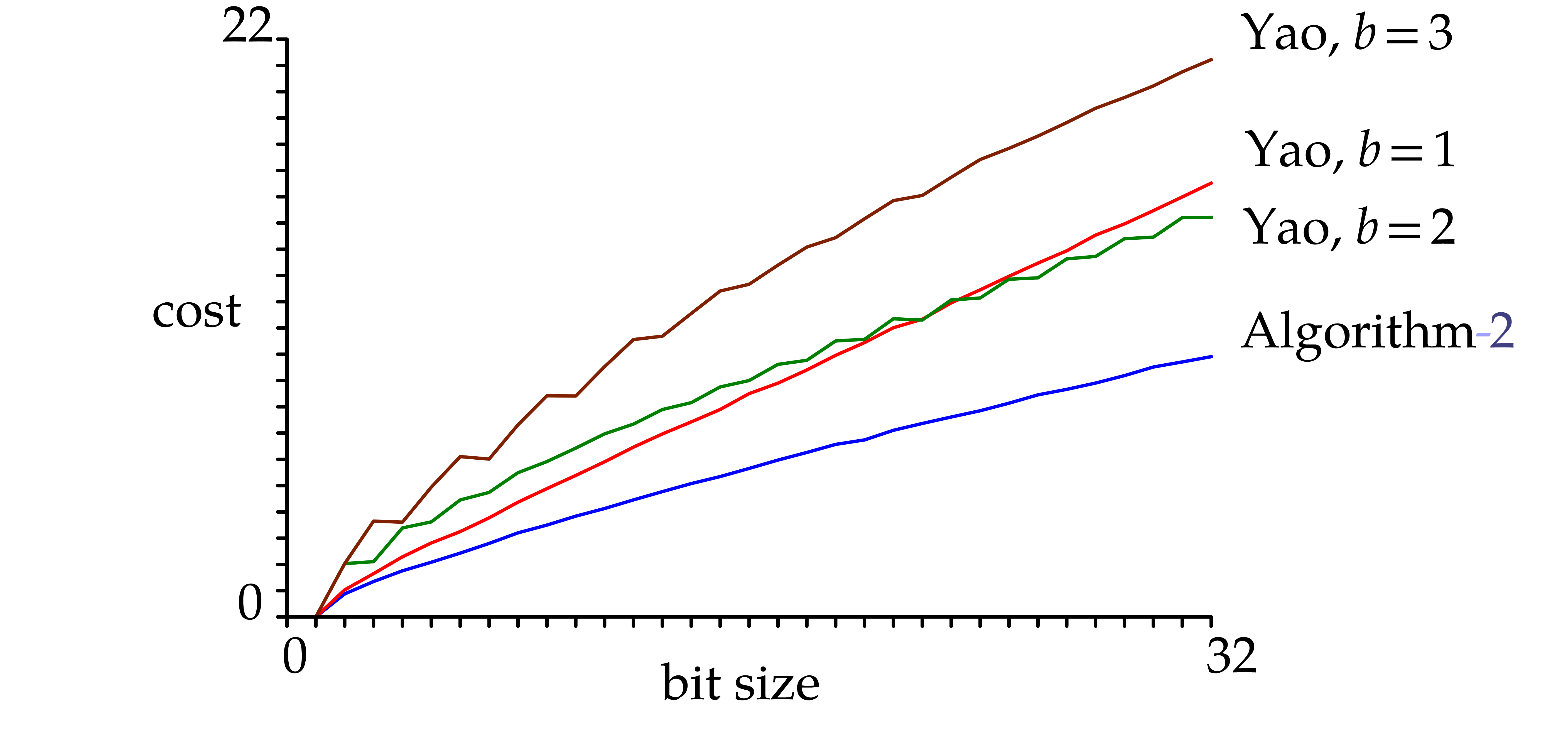Figure 1. Computation of several powers using Yao's method and Algorithm 2.

The original condition and the weakened condition show that Yao's method is mostly of theoretical interest. For practical purposes, we therefore designed Algorithm 2 below, based on ‑adic expansions. It incorporates opportunistic optimizations whenever possible. As shown in Figure 1, this algorithm improves upon Yao's method for the exponent sizes that we are interested in.

Example 1. Taking , Algorithm 2 returns the addition chain . An optimal addition chain is .

Remark 2. Given , the problem of finding the absolute shortest addition chain with is known to be NP-complete [10].

2.3.Multiple power products

The -adic approach can also be used for the computation of power products. This was already realized by Straus [23], who showed that can be computed using multiplications, where , and provided that . The similarity between the complexities of Straus' and Yao's algorithms is not accidental, since both problems are equivalent due to a suitable application of the transposition principle. For more details and historical references, we refer to Bernstein's survey [2].

Another interesting observation due to Straus is that, for the computation of a single power product , the naive strategy to compute and multiply is typically not the fastest. In our implementation, for small exponents, we found it simpler to simultaneously replace all powers that occur in our vector of sparse polynomials by new variables. For each variable , this requires us to call Algorithm 2 for the list of all exponents such that occurs in . Consequently, we do not benefit from the additional improvements that Straus provides for large exponents; however, we describe an alternate practical strategy in section 3.2.

In fact, Pippenger also proposed an algorithm [20, 21, 22] for evaluating multiple power products . This algorithm is more elaborate to implement and we again refer to Bernstein's survey [2] for an overview. In section 3.4, we will present an efficient and easily implementable alternative for a key step in Pippenger's algorithm for the case when for all .

2.4.Multivariate Horner schemes

Let us now return to the problem of computing an SLP for evaluating a single sparse polynomial (1). In computer algebra systems, sparse polynomials are often represented recursively as polynomials in a single variable , whose coefficients are sparse polynomials in the remaining variables . This allows us to evaluate each of the univariate polynomials in this representation using Horner's method (or using a variant of Horner's method if the univariate polynomials are themselves represented in a sparse manner).

Another option is to decompose with and where some of the terms may be zero and left out. We may then recursively expand in a similar manner. Of course, we may also impose additional constraints on . For instance, if is our main expansion variable as above, then we may require not to depend on .

Such multivariate Horner schemes have been studied in several works [6, 7]. One major issue concerns the choice of the main expansion variable and the subsequent choices of the main expansion variables for all recursive coefficients.

In lucky cases, typically when the support of is rather dense, multivariate Horner schemes may return an SLP of size . However, on many examples from our data base, the size of the computed SLP is closer to . Multivariate Horner schemes nonetheless remain a good “naive way” to evaluate sparse polynomials, since they are easy to implement and always outperform brute force evaluation of the expression (1).

2.5.Bilinear schemes

Consider a sparse polynomial with support . If has a “dense flavor”, then it is often possible to subdivide the set of variables into two subsets, say and , in such a way that the projected supports

are significantly smaller than . For instance, if is a generic polynomial in variables of total degree , so that , then and . If is fixed and , then this yields and

In this favorable situation, we may first compute the power products for all , as well as the power products for all , and then deduce all power products for using only additional multiplications. Assuming that , the entire evaluation of can then be done using multiplications and FMA instructions; Here an FMA instruction is of the form . One may view this method as re-interpreting as a bilinear polynomial in the variables and .

Remark 3. Although this scheme is not expected to be efficient for general purposes, it becomes very attractive whenever the ring operations in can be performed in a suitable FFT model or using modular arithmetic. In that case, the transforms (FFT transforms or modular reductions) of the coefficients can be precomputed. For the evaluation of , we then compute the power products and as above, along with their transforms. We next do the multiplications in the transformed model, as well as all the FMAs. We finally transform the result back to the final value in . The bulk of the computation then reduces to multiplications and FMAs in the transformed model. This technique was proposed in [13, section 4.4.3].

Example 4. Assume that is a ring of power series over a field and assume that the are actually in . Assuming that contains a primitive root of unity of smooth order , then we may use FFTs of length to transform elements of into vectors in . If the are in , then we rather need an of smooth order instead. If we subdivide our set of variables into instead of two sets, then similar ideas still apply, but we need an of smooth order . Similar remarks apply for modular arithmetic.

2.6.Partial factorizations

The smallest SLP that evaluates a given sparse polynomial may be much smaller than the input polynomial. One example is the polynomial

(2)

from the introduction, where and can be computed using repeated squarings. Unfortunately, finding such SLPs from their expanded representations is very hard in general. Nonetheless, it is often possible to find at least some partial factorizations that may help to speed up the evaluation.

The problem of factoring sparse polynomials in the traditional mathematical sense has been studied extensively. We refer to [9] for some recent algorithms and historical references. However, the kind of “factorizations” as in (2) that we are really after are not exclusively multiplicative, but may involve both additions and multiplications. In fact, the multivariate Horner schemes that we discussed in section 2.4 can be regarded as easy-to-compute additive-multiplicative factorizations, by recursively factoring out single variables. We will also use this kind of factorizations in section 3.3 below.

In [18], a reasonably efficient algorithm has been presented for finding “syntactic factorizations”, in which none of the terms of the expanded products and sums overlap. For instance, is a syntactical factorization of , but is not a syntactical factorization of , because of the two “overlapping” terms and . The algorithm from [18] works well for applications in which syntactic factorizations are likely to occur, such as input polynomials that are themselves the expanded result of some algebraic computation (in [18] a generic resultant was used as the running example).

In this paper, we focus on SLP transforms which can be computed in quasi-linear time or almost, so we regard the computation of more clever additive-multiplicative factorizations as a more or less independent problem to which we plan to return in future work.

3.The new algorithm

Let be the input variables. Consider a vector of sparse polynomials with

In this section, we present our main algorithm to compute an SLP for the efficient evaluation of as a polynomial map. In brief, our algorithm proceeds as follows:

1. All powers of individual variables are evaluated and replaced with new variables; coefficients are also replaced by new variables. Consequently, each term of the polynomial is expressed as a product of distinct variables.

2. Horner‑type factorizations are applied to the polynomials obtained in step 1.

3. We collect all remaining products of distinct variables that need to be evaluated and use a greedy algorithm to evaluate them simultaneously.

4. The final straight‑line program is then simplified and optimized for the target hardware.

3.1.Replacing coefficients and powers by new variables

The first step of our algorithm is a reduction to the case where and for all . We do this by first introducing new variables for all constants . Whenever a constant occurs multiple times, we understand that we introduce a single variable to represent all these identical constants.

For each variable , we next collect the set of all non-zero exponents such that occurs in one of the terms of one of the . All sets can be determined jointly using a hash table and one linear pass. Whenever , we next use Algorithm 2 to compute an addition chain for the sorted list of elements of . This addition chain gives rise to an SLP of the same length minus one for the computation of for all . For each with , we introduce a new variable , and use the latter SLPs to compute these new variables as a function of .

Example 5. As our running example, consider and

(3)

We first introduce new variables and for the constants. We next need to introduce new variables for all non-trivial powers. For the variable , we need to compute and , which we do using Algorithm 2. This yields , , , so and . We next need to compute , , , and , which is done as follows: , , , , , . We finally need to compute and , which is done using , . After the introduction of these new variables, our sparse polynomials are rewritten as

(4)

3.2.Binary expansion of exponents

We have just shown how to reduce our evaluation problem to the case where all input polynomials

are sums of products of distinct variables. Instead of introducting a distinct variable for each individual power , it is also possible to further factor such powers as products of powers of the form . For this, we compute the -adic expansions of the exponents

Setting , we then have

(5)

As in the previous subsection, we introduce new variables for the coefficients , whereas the evaluation of the is done directly using binary exponentiation instead of Algorithm 2.

3.3.Factoring out variables in a greedy manner

After applying one of the two rewriting algorithms described in the previous subsections, the input polynomials become sums of products of variables. Although finding the best possible partial factorizations is a hard problem in general, we still can go for “low hanging fruit”, by recursively factoring out single variables from the polynomials as long as possible.

More precisely, for each polynomial , let be a variable such that the number of terms that depend on is maximal. If and for some small number (say ), then we decompose and replace by the two polynomials and in the list (or just by if ). We keep doing this until no such exists. Due to the threshold , this algorithm runs in quasi-linear time.

Example 6. Applying this strategy to the polynomials (4) leads to the factorizations

The algorithm of the next subsection will compute the values of , , , , , , into the variables , , , , , , ; see Example 9. In order to compute and it remains to perform the following instructions:

After this, we have and . Here .

3.4.Greedy evaluation of a list of products

In this subsection, we turn to the core subalgorithm. As input, we have a list of pairwise distinct subsets of . As output, we produce an SLP that takes as input and that computes for . Without loss of generality we may assume that .

For the construction of our SLP we use a simple greedy approach: as long as the list contains two entries with , we determine variables , for which is maximal. We then introduce a new variable and replace by in the subsets and increase by one. As soon as for all , the products all become trivial. The algorithm runs as follows.

Proof. Let . Steps 2 and 3 perform operations on integers of bit size . If holds in step 4b, then the triple is no longer valid. Let denote the value of at the end of the algorithm.

The bit cost of each update caused by in step 4d is . Moreover, each can be updated at most times. Consequently, . Hence, the total cost is .

Remark 8. In practice a hash table is used for in Algorithm 3. Assuming perfect hashing the asymptotic complexity is the same.

Example 9. Continuing our Example 6, let us take

(6)

The two variables and appear jointly in two of the . The algorithm starts by picking in step 4a, so we append to the SLP, and also update , , and the table . We next pick in step 4a, append to the SLP, and also update , , and the table . We next pick from the heap, but since has been updated to , we ignore this pick in step 4b and directly continue with the next triple on the heap. From this point on, we only retrieve triples with and further append the following instructions to the SLP (while indicating their values in terms of in grey):

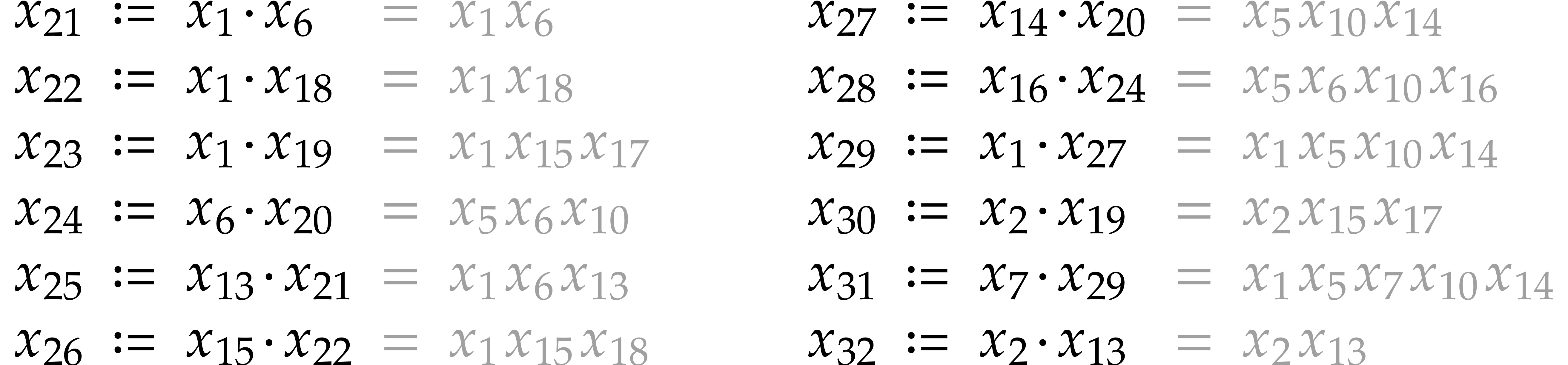
The output variables are , , , , , , .

3.5.Simplification and polishing

As our final step, we try to combine as many additions with multiplications as possible into FMA instructions, and run common subexpression elimination on the result. Optionally, we may reschedule some of the instructions and try to reduce the number of variables that are being used.

Example 10. For our running Example 5, it is possible to group two pairs of additions and multiplications into FMA instructions. We may also rewrite multiplications as squarings (which is more efficient for certain rings ). On the other hand, common subexpression elimination leads to no further simplifications. The final SLP is:

4.Implementation

We implemented our new algorithm within the JIL library [1, 15], GIT version d390808a9b9834f64a73bb823d7745cd806c0dc0. JIL is a free C++ software library for HPC computations with SLPs. It provides a convenient interface for automatic differentiation, common sub-expression elimination, lifting, transposition, and many other features. It also includes a JIT (Just In Time) compiler dedicated to SLPs. This compiler can generate executable machine code directly in memory, which is useful when the same SLP needs to be evaluated multiple times efficiently. Typical applications include numerical integration and polynomial system solving.

The JIT compiler of JIL is one or two orders of magnitude faster than general‑purpose compilers such as GCC or CLANG. Consequently, JIT compilation becomes advantageous even for relatively small values of like . In addition, if several competing SLPs are available for the same task, then we can generate machine code for each of them and empirically select the best SLP.

The source code of our evaluation can be found in the file src/slp/slp_spol.cpp of JIL. Examples are in check/slp/slp_spol_check.cpp and benchmarks in bench/slp/slp_spol_bench.cpp.

4.1.Implemented strategies

Currently, our implementation supports 32-bit integer exponents represented by sparse vectors. The SLPs produced by our software include the following operations: negation, binary addition, subtraction, and possibly negated multiplication , as well as ternary FMA instructions . Our goal is to minimize the length (i.e. the number of operations) of the generated SLP. Below we analyze the obtained results for the following strategies.

Sparse

This strategy corresponds to our new polynomial evaluation algorithm from section 3, while using the algorithm from section 3.1 for the reduction to the case of sums of powers of distinct variables.

Exponent expansion

This is a variant of the “sparse” strategy in which we use the algorithm from section 3.2 instead of the one from section 3.1.

Horner

Here, the input polynomial is considered in , where maximizes the number of distinct exponents of among the non-zero terms of :

(7)

We apply this Horner strategy recursively to evaluate all the . Then the univariate Horner scheme is applied to obtain the value of using

The powers are computed using Algorithm 2.

Greedy Horner

We have implemented an improved variant of the strategy presented in [7, section 3]: selecting the variable as in the above “Horner” strategy, we write

where contains all the terms of that are not multiple of and is not divisible by . The polynomials and are evaluated recursively. We collect all powers from all recursive evaluations upfront and evaluate them using Algorithm 2.

4.2.Sparse random polynomials

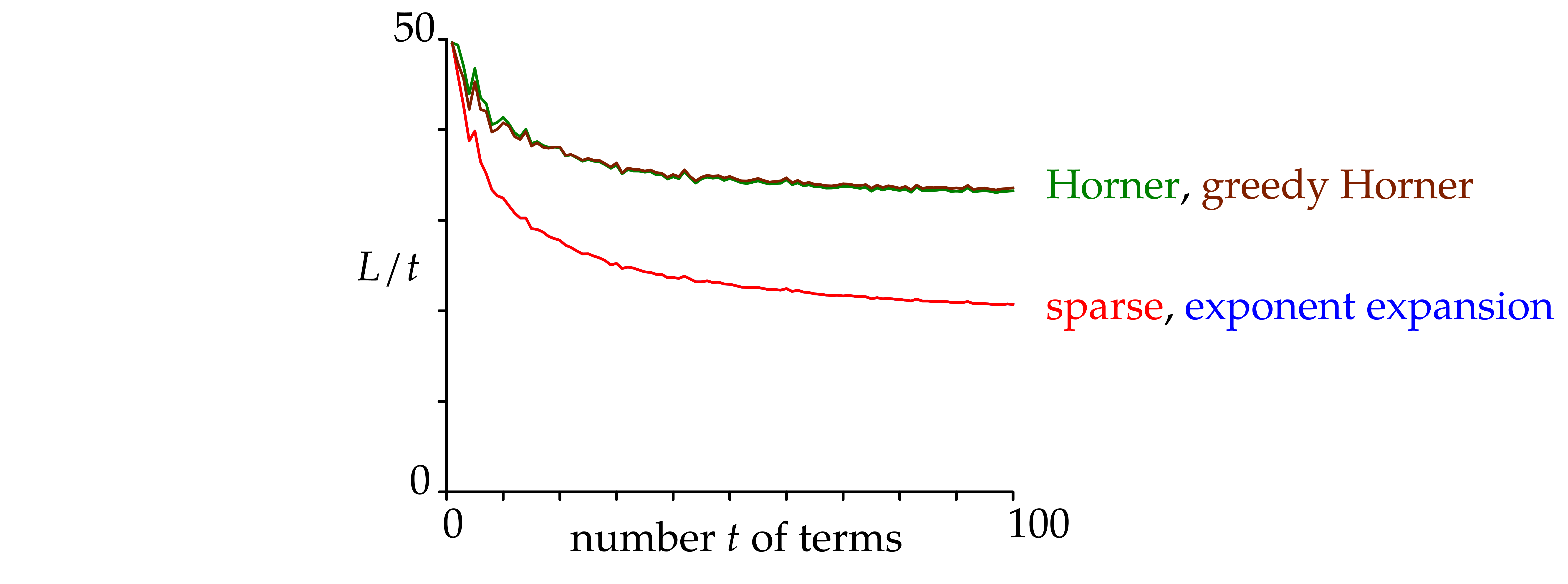
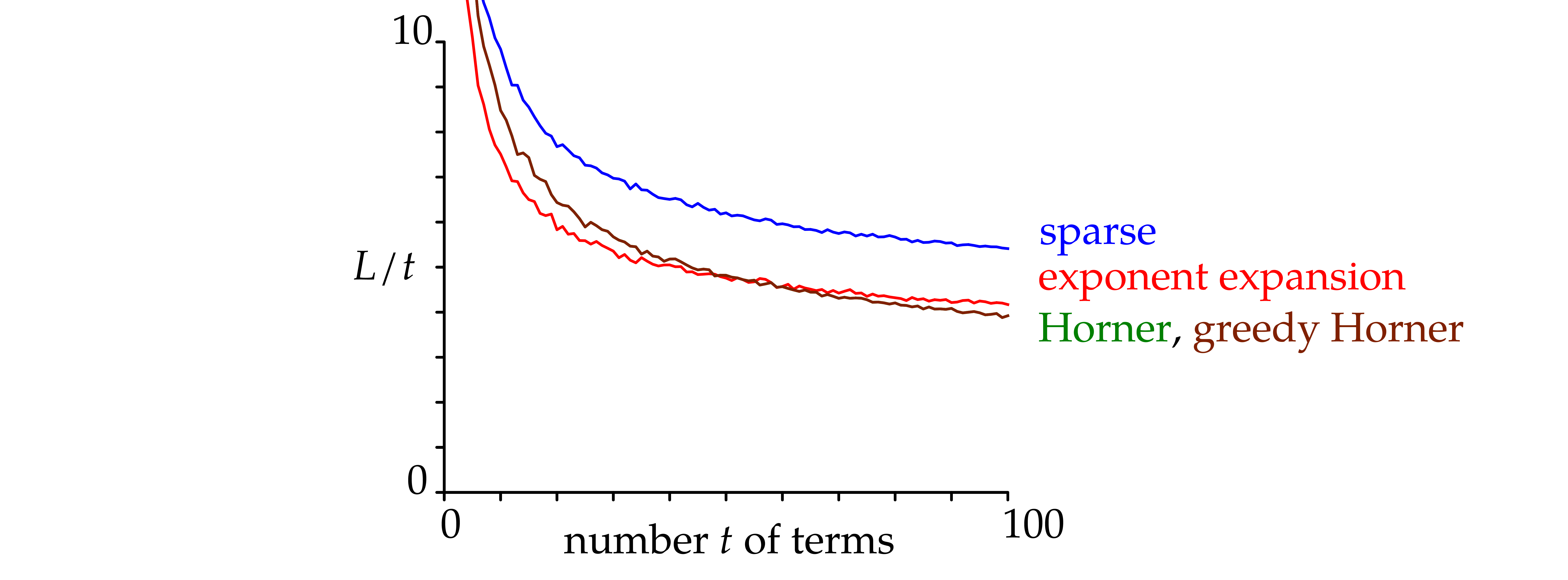
The strategies from section 3 were designed specifically for polynomials with few terms of small degree. In particular, we considered the case of random polynomials with terms in variables and exponents in . Figure 2 displays the length of the generated SLP divided by as a function of . The cost is averaged over 10 random samples. The costs of the “sparse” and “exponent expansion” strategies are actual identical in this special case. Those of “Horner” and “greedy Horner” are almost the same.

Figure 2. Ratio as a function of , where is the length of the SLP generated using different strategies, for random polynomials with terms in variables and exponents in .

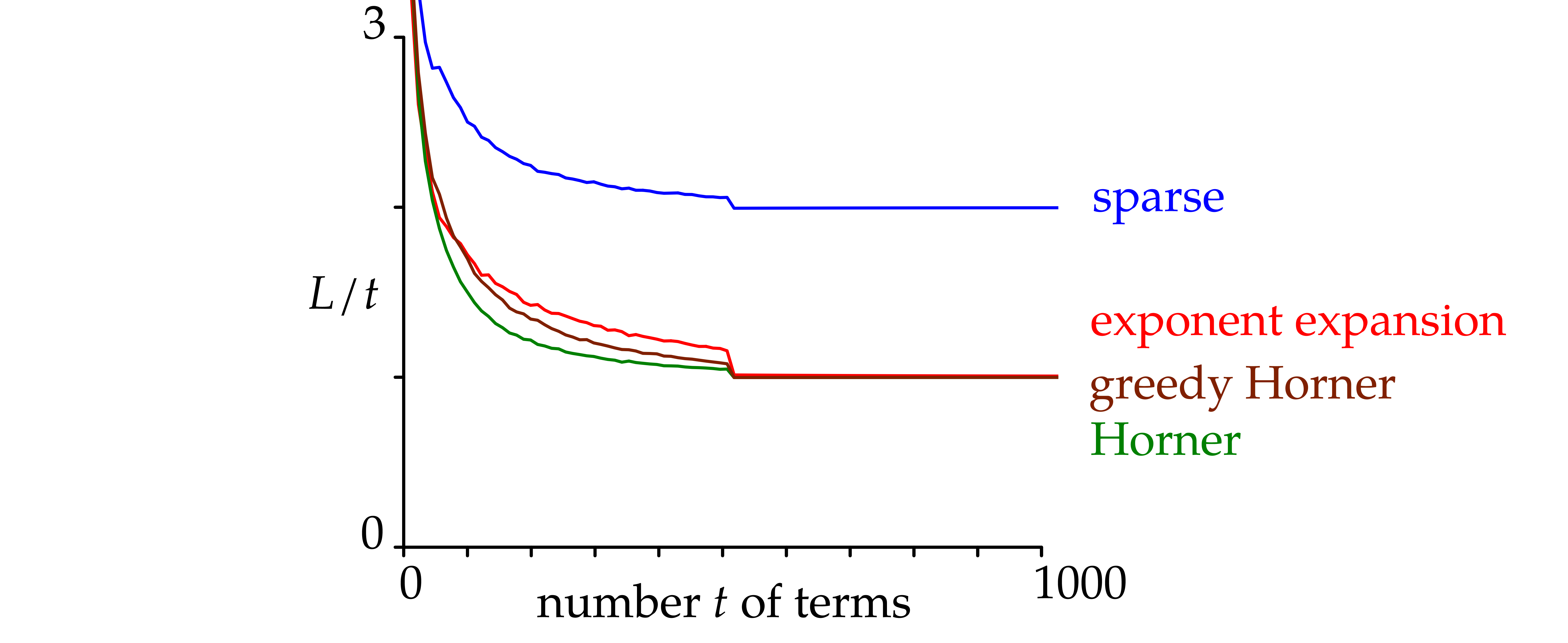
Figure 3 displays similar cost measures with and exponents constructed randomly as follows: we first select a bit size in at random and then pick a random number uniformly in . We observe that the “sparse” strategy is ineffective. With fewer than about 50 terms, the “exponent expansion” strategy performs best; thereafter, the “Horner” strategy (which coincides with the “greedy Horner” strategy) becomes more efficient. With a few variables (e.g., 2, 3, 4), the comparisons are similar, with larger thresholds ( becomes approximately for ).

Figure 3. Ratio as a function of , where is the length of the SLP generated using different strategies, for random univariate polynomials of degree with terms.

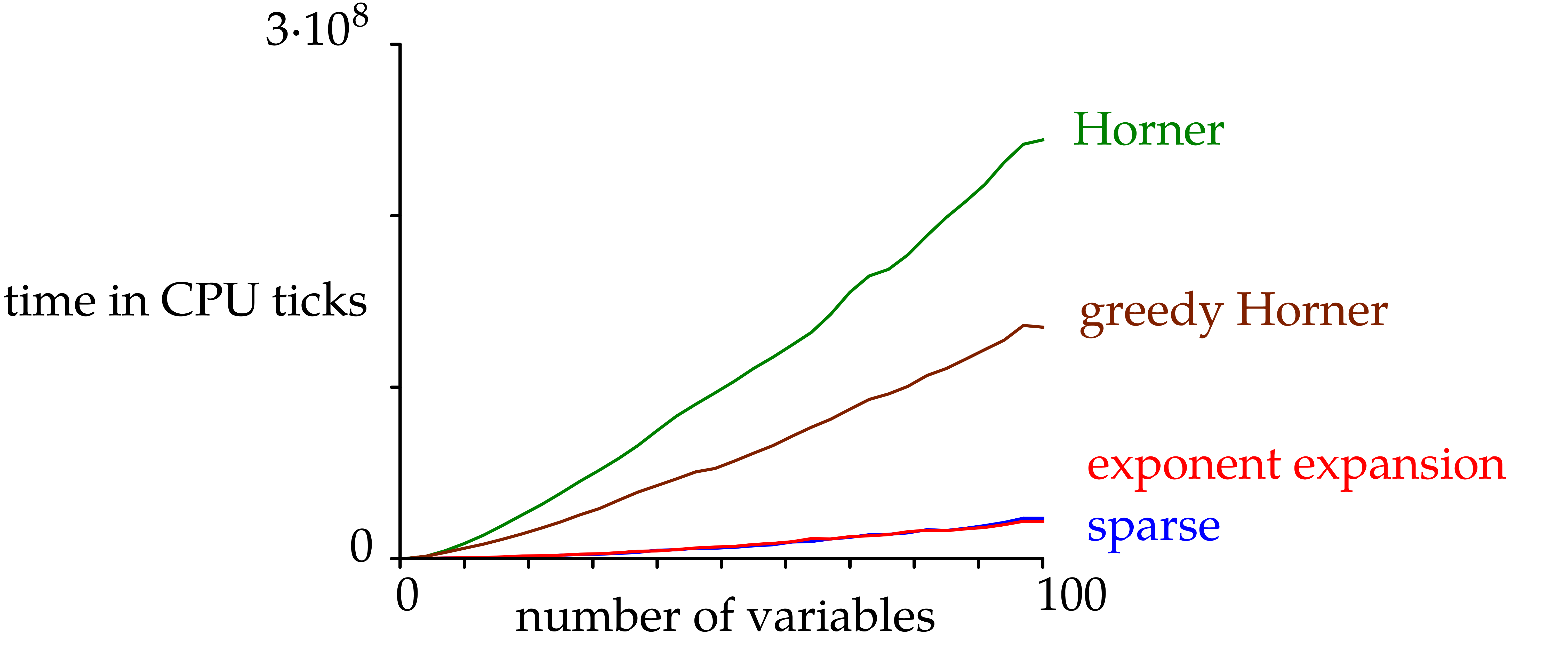
Figure 4 displays the time needed to build the SLPs using the four strategies: we construct polynomials in variables with at most 100 terms and random exponents in . Coefficients are random 64 bit integers. The cost is averaged over 10 random samples. We observe that the Horner strategies are considerably less efficient than the sparse strategies when the number of variables is large.

Figure 4. Times for builing SLPs of random polynomials with terms and coefficients in .

4.3.Dense polynomials

The “Horner” and “greedy Horner” strategies coincide for univariate polynomials and are usually the most efficient. The “exponent expansion” method is only slightly slower, while the “sparse” strategy is suboptimal in this situation. Figure 5 shows averaged ratios as a function of (for random samples), this time for random bivariate dense polynomials of partial degrees . The behavior is roughly similar to what we observed in the univariate case. For trivariate polynomials of partial degrees , the four strategies have closer efficiencies.

Figure 5. Ratio as a function of , where is the length of the SLP generated using different strategies, for random bivariate polynomials of partial degrees .

4.4.Our final “combined” strategy

Considering the relative performance of the four strategies described above, and noting that the construction of an SLP via the Horner methods tends to become more expensive for sparse polynomials, we retained a “combined” default strategy for the evaluation of sparse polynomials in JIL. More precisely, our implementation selects the shortest SLP among the ones produced via the following strategies:

1. The first strategy is “exponent expansion”.

2. The second strategy performs a single step of the “Horner” strategy (i.e. with respect to a single variable), followed by the “exponent expansion” strategy (where we evaluate all the of equation (7) simultaneously).

3. The third strategy performs two steps of the “Horner” strategy, followed by the “exponent expansion” strategy: after the first step of the “Horner” strategy and we evaluate all the of (7) simultaneously using the second strategy. All the are considered as univariate polynomials in the same variable , where maximizes the number of distinct exponents of among the union of the non-zero terms of . Of course, we only apply this third strategy when the second strategy produces a shorter SLP than the first one.

This “combined” strategy is almost always best for sparse multivariate polynomials. For denser polynomial, it still performs well, since the density is typically captured by one and sometimes two of the variables. The most expensive step of computing the SLP using the “combined” strategy is Algorithm 3. The other steps run in quasi‑linear time.

To benchmark the efficiency of our “combined” strategy, we collected polynomial systems with integer coefficients primarily from the SymbolicData project [ 12 ] and the msolve example suite [ 3 ]. These systems are available at https://sourcesup.renater.fr/projects/jil-examples . We measured the lengths , , and of the SLPs produced by the “combined”, “Horner”, and “greedy Horner” strategies. In Figure 6 , each polynomial system is represented by a cross: the abscissa shows the logarithm of the bit size of the system, and the ordinate shows .

Figure 6. Relative performance of the “combined” strategy across the database.

After a closer examination of the timings, we observed that relatively dense homogeneous bivariate polynomials are better suited for the “exponent expansion” method than for Horner's method. On the other hand, the points with low ordinates in Figure 6 often correspond to systems with a very specific structure, for example those labeled Singular_rcyclic in the database. These rare cases are where the “greedy Horner” method outperforms “combined”. Of course, in our software implementation, the user can select the strategy and even invoke an intensive search for optimal combinations. We are also investigating variants of our algorithms that use more aggressive factorizations in the same vein as [18]. We plan to detail this work in a future paper.

Bibliography