Abstract

In this paper, we consider the problem of efficient computations with structured polynomials. We provide complexity results for computing Fourier Transform and Truncated Fourier Transform of symmetric polynomials, and for multiplying polynomials supported on a lattice.

1.Introduction

Fast computations with multivariate polynomials and power series have been of fundamental importance since the early ages of computer algebra. The representation is an important issue which conditions the performance in an intrinsic way; see [23, 31, 8] for some historical references.

It is customary to distinguish three main types of representations: dense, sparse, and functional. A dense representation is made of a compact description of the support of the polynomial and the sequence of its coefficients. The main example concerns block supports – it suffices to store the coordinates of two opposite vertices. In a dense representation all the coefficients of the considered support are stored, even if they are zero. If a polynomial has only a few non-zero terms in its bounding block, we shall prefer to use a sparse representation which stores only the sequence of the non-zero terms as pairs of monomials and coefficients. Finally, a functional representation stores a function that can produce values of the polynomials at any given point. This can be a pure blackbox (which means that its internal structure is not supposed to be known) or a specific data structure such as straight-line programs (see Chapter 4 of [4], for instance, and [10] for a concrete library for the manipulation of polynomials with a functional representation).

For dense representations with block supports, it is classical that the algorithms used for the univariate case can be naturally extended: the naive algorithm, Karatsuba's algorithm, and even Fast Fourier Transforms [7, 30, 6, 28, 16] can be applied recursively in each variable, with good performance. Another classical approach is the Kronecker substitution which reduces the multivariate product to one variable only; for all these questions, we refer the reader to classical books such as [29, 14]. When the number of variables is fixed and the partial degrees tend to infinity, these techniques lead to softly linear costs.

After the discovery of sparse interpolation [2, 24, 25, 26, 11], probabilistic algorithms with a quasi-linear complexity have been developed for sparse polynomial multiplication [5]. It has recently be shown that such asymptotically fast algorithms may indeed become more efficient than naive sparse multiplication [19].

In practice however, it frequently happens that multivariate polynomials with a dense flavor do not admit a block support. For instance, it is common to consider polynomials of a given total degree. In a recent series of works [15, 17, 18, 21, 20], we have studied the complexity of polynomial multiplication in this “semi-dense” setting. In the case when the supports of the polynomials are initial segments for the partial ordering on , the truncated Fourier transform is a useful device for the design of efficient algorithms.

Besides polynomials with supports of a special kind, we may also consider what will call “structured polynomials”. By analogy with linear algebra, such polynomials carry a special structure which might be exploited for the design of more efficient algorithms. In this paper, we turn our attention to a first important example of this kind: polynomials which are invariant under the action of certain matrix groups. We consider only two special cases: finite subgroups of and finite groups of diagonal matrices. These cases are already sufficient to address questions raised e.g. in celestial mechanics [12]; it is hoped that more general groups can be dealt with using similar ideas.

In the limited scope of this paper, our main objective is to prove complexity results that demonstrate the savings induced by a proper use of the symmetries. Our complexity analyses take into account the number of arithmetic operations in the base field, and as often, we consider that operations with groups and lattices take a constant number of operations. A serious implementation of our algorithms would require an improved study of these aspects.

Of course, there already exists an abundant body of work on some of these questions. Crystallographic FFT algorithms date back to [32], with contributions as recent as [27], but are dedicated to crystallographic symmetries. A more general framework due to [1] was recently revisited under the point of view of high-performance code generation [22]; our treatment of permutation groups is in a similar spirit, but to our understanding, these previous papers do not prove results such as those we give below (and they only consider the FFT, not its truncated version).

Similarly, our results on diagonal groups, which fit in the general context of FFTs over lattices, use similar techniques as in a series of papers initiated by [13] and continued as recently as [33, 3], but the actual results we prove are not in those references.

2.The classical FFT

2.1Notation

We will work over an effective base field (or ring) with sufficiently many roots of unity; the main objects are polynomials in variables over . For any and , we denote by the monomial and by the coefficient of in . The support of a polynomial is the set of exponents such that .

For any subset of , we define as the polynomials with support included in . As an important special case, when , we denote by the set of polynomials with partial degree less than in all variables.

Let be a primitive th root of unity (in Section 4, it will be convenient to write this root ). For any , we define . One of our aims is to compute efficiently the map

when is a “structured polynomial”. Here, denotes the set of vectors with entries in indexed by ; in other words, implies that for all . Likewise, denotes the set of matrices with indices in , that is, implies that for all .

Most of the time, we will take with , although we will also need more general of mixed radices .

We denote by the inner product of two vectors in . We also let , for , be the th element of the canonical basis of . At last, for and we denote by the bit reversal of in length and we extend this notation to vectors by .

2.2The classical multivariate FFT

Let us first consider the in-place computation of a full -dimensional FFT of length in each variable. We first recall the notations and operations of the decimation in time variant of the FFT, and we refer the reader to [9] for more details. In what follows, is a th primitive root of unity.

We start with the FFT of a univariate polynomial . Decimation in time amounts to decomposing into its even and odd parts, and proceeding recursively, by means of decimations applied to the variable . For , we will write for the input and denote by the result after decimation steps, for .

At stage , the decimation is computed using butterflies of span . If is even and belongs to then these butterflies are given by

Putting the coefficients of all these linear relations in a matrix , we get . The matrix is sparse, with at most two non-zero coefficients on each row and each column; up to permutation, it is block-diagonal, with blocks of size 2. After stages, we get the evaluations of in the bit reversed order:

We now adapt this notation to the multivariate case. The computation is still divided in stages, each stage doing one decimation in every variable . Therefore, we will denote by the coefficients of the input for and by the coefficients obtained during the th stage, after the decimations in are done, with and , so that . We abbreviate for the coefficients after stages.

The intermediate coefficients can be seen as evaluations of intermediate polynomials: for every , and , one has

(1)

where are obtained through an -fold decimation of . Equivalently, the coefficients satisfy

(2)

Thus, yields in bit reversed order.

For the concrete computation of the coefficients at stage from the coefficients at stage , we use so called “elementary transforms” with respect to each of the variables . For any , the coefficients are obtained from the coefficients through butterflies of span with respect to the variable ; this can be rewritten by means of the formula

(3)

for any with even -th coordinate and . Equation (3) can be rewritten more compactly in matrix form where is a sparse matrix in which is naturally indexed by pairs of multi-indices in . Setting we also obtain a short formula for as a function of :

(4)

Remark that the matrices commute pairwise. Notice also that each of the rows and columns of has at most non zero entries and consequently those of contains at most non zero entries. For this reason, we can apply the matrices (resp. ) within (resp. ) operations in . Finally, the full -dimensional FFT of length costs operations in (see [14, Section 8.2]).

Example 1. Let us make these matrices explicit for polynomials in variables and degree less than , so that . We start with the first decimation in whose butterflies of span are captured by with and . It takes as input and outputs for . For any and , we let

So, is a 16 by 16 matrix, which is made of diagonal blocks of in a suitable basis. The decimation in during stage is similar :

for and . Consequently, is made of diagonal blocks (in another basis than ). Their product corresponds to the operations

for . Thus is made of such 4 by 4 matrices on the diagonal (in yet another basis). Note that in general, the matrices and are still made of diagonal blocks, but these blocks vary along the diagonal.

We can sum it all up in the two following algorithms.

Algorithm Butterfly Input: , degree , stage , index of the butterfly with , , root of unity and coefficients for the butterfly ( for ). Output: the output of the butterfly

For do //decimation in For such that do //butterfly in one variable Return

Algorithm FFT Input: , degree , and coefficients of Output: coefficients in bit reversed order

For do //stage For , do //pick a butterfly For do For do Return

In the last section, we will also use the ring isomorphism

with for , and . These polynomials generalize the decomposition of a univariate polynomials into and . We could obtain them through a decimation in frequency, but it is enough to remark that we can reconstruct them from the coefficients thanks to the formula

(5)

3.The symmetric FFT

In this section, we let be a permutation group. The group acts on the polynomials via the map

We denote by the set of polynomials invariant under the action of . Our main result here is that one can save a factor (roughly) when computing the FFT of an invariant polynomial. Our approach is in the same spirit as the one in [1], where similar statements on the savings induced by (very general) symmetries can be found. However, we are not aware of published results similar to Theorem 7 below.

3.1The bivariate case

Let be a symmetric bivariate polynomial of partial degrees less than , so that ; let also be a primitive eighth root of unity. We detail on this easy example the methods used to exploit the symmetries to decrease the cost of the FFT.

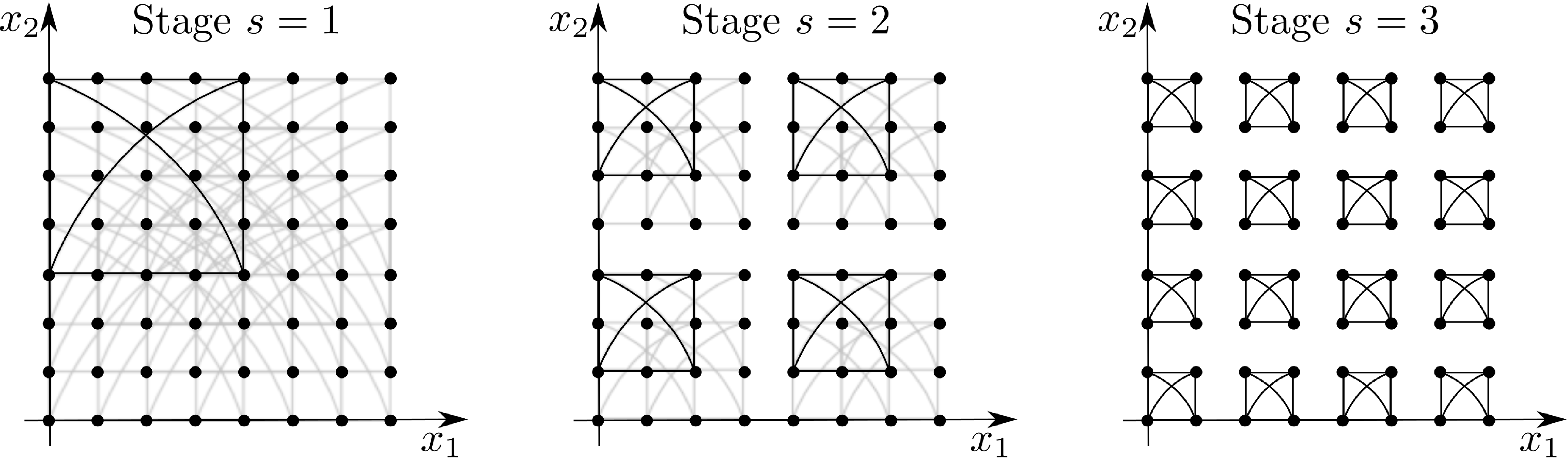
The coefficients of are placed on a grid. The bivariate classical FFT consists in the application of butterflies of size for from to , as in Figure 1. When some butterflies overlap, we draw only the shades of all but one of them. The result of stage is the set of evaluations in bit reversed order.

Figure 1. Classical bivariate FFT

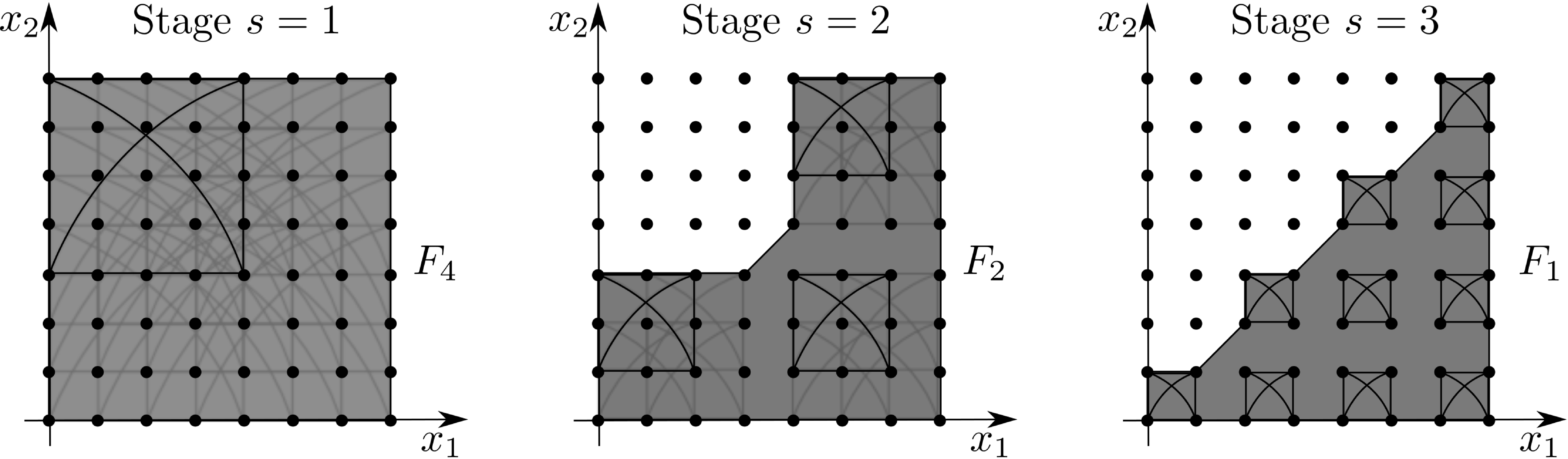
We will remark below that each stage preserves the symmetry of the input. In particular, since our polynomial is symmetric, the coefficients at stage are symmetric too, so we only need to compute the coefficients for in the fundamental domain (sometimes called asymmetric unit) . We choose to compute at stage only the butterflies which involves at least an element of ; the set of indices that are included in a butterfly of span that meets will be called the extension of .

Figure 2. Symmetric bivariate FFT

Every butterfly of stage meets the fundamental domain, so we do not save anything there. However, we save out of butterflies at stage and out of butterflies at the third stage. Asymptotically in , we gain a factor two in the number of arithmetic operations in compared to the classical FFT; this corresponds to the order of the group.

3.2Notation

The group also acts on with for any . This action is consistent with the action on polynomials since .

Because acts on polynomials, it acts on the vector of its coefficients. More generally, if and , we denote by the vector defined by for all . If is stable by , i.e. , we define the set of invariant vectors by .

For any two sets satisfying , we define the restriction of by for all . Recall the definition of the lexicographical order : for all , if there exists such that for any and . Finally for any subset stable by , we define a fundamental domain of the action of on by together with the projection such as .

3.3Fundamental domains

Let be the fundamental domain associated to the action of on . Any -symmetric vector can be reconstructed from its restriction using the formula . As it turns out, the in-place FFT algorithm from Section 2.2 admits the important property that the coefficients at all stage are still -symmetric.

Lemma 2. Let and the vectors be as in Section 2.2. Then if , .

Proof. Given , and , we clearly have . For any , , and , we also notice that

Hence, using Equation (2), we get

Thus, for all , whence .

This lemma implies that for the computation of the FFT of a -symmetric polynomial , it suffices to compute the projections .

In order to apply formula (4) for the computation of as a function of , it is not necessary to completely reconstruct , due to the sparsity of the matrix . Instead, we define the -expansion of the set by

where stands for the “bitwise exclusive or” of and . For any , the set describes the vertices of the butterfly of span that includes the point . Thus, is indeed the set of indices of that are involved in the computation of via the formula .

Lemma 3. For any , let

so that . Then we have .

Proof. Assume that . Then clearly, , whence . Conversely, if , then there exists a with and . Let . For any , we have . Consequently, , whence .

For the proof of the next lemma, for , define and

Lemma 4. There exists a constant (depending on ) such that

Proof. With the notation above, we have . Taking , it follows that . On the other hand, the orbit of any element in under contains exactly elements and one element in . In other words, and so . Finally, which implies .

3.4The symmetric FFT

Let be the restriction of to and notice that is stable under , i.e. . Therefore the restriction of the map to vectors in is a -algebra morphism from to . By construction, we now have This allows us to compute as a function of using

(6)

where denotes the -expansion of .

Remark 5. We could have saved a few more operations by only computing the coefficients . To do so, we would have performed just the operations of a butterfly corresponding to vertices inside . However, the potential gain of complexity is only linear in the numbers of monomials .

The formula (6) yields a straightforward way to compute the direct FFT of a -symmetric polynomial:

Remark 6. The main challenge for an actual implementation of our algorithms consists in finding a way to iterate on sets like without too much overhead. We give a hint on how to iterate over in Lemma 8 (see also [22] for similar considerations).

The inverse FFT can be computed classically by unrolling the loops in the inverse order and inverting the operations of the butterflies. The main result of this section is then the following theorem, where denotes the cost of a full -dimensional FFT of multi-degree .

Theorem 7. For fixed and , and for , the direct (resp. inverse) symmetric FFT can be computed in time

Proof. At stage of the computation, the ratio between the computation of as a function of and as a function of is , so that

Lemmas 3 and 4 thus imply

whence

The result follows for .

Finally, the following lemma gives a description of an “open” subset of , characterized only by simple inequalities. Although we do not describe implementation questions in detail here, we point out that this simple characterization would naturally be used in order to iterate over the sets , possibly using tree-based techniques as in [17].

Lemma 8. Let be the set of such that and such that for and . For , define . Then

Proof. Assume that does not lie in . Then for some . Let be minimal with , whence and . Since , it follows that , so . Inversely, assume that does not lie in , so that there exists with . Let be such that for and . Then, .

4.The lattice FFT

In this section, we deal with polynomials supported on lattices; our main result is an algorithm for the multiplication of such polynomials using Fourier transforms.

The first subsection introduces the main objects we will need (a lattice and its dual ); then, we will give an algorithm, based on Smith normal form computation, for the FFT on what we will call a basic domain, and we will finally deduce a multiplication algorithm for the general case.

The techniques we use, based on Smith normal form computation, can be found in several papers, originating from [13]; in particular, the results in Section 4.2 are essentially in [33] (in a more general form).

4.1Lattice polynomials

Assume that admits a primitive th root of unity for any order , which we will denote by . Let be a free -submodule of of rank , generated by the vectors . Then

is a subring of , and we will call elements of lattice polynomials. First, we show that these polynomials are the invariant polynomial ring for a diagonal matrix group.

The set acts on via, for any , the isomorphism of given by

Note that for any . The action of on the monomial is given by .

In particular, all elements of are invariants under the action of if and only if

(7)

where is the matrix with columns , that is . Let be the dual (or reciprocal) lattice of , that is the set of all satisfying Equation (7). A basis of is given by the columns of .

Let be the group of actions . It is generated by , where are the columns of . From Equation (7), we deduce that is the diagonal matrix group of all actions which leave invariant. Conversely, because monomials are mapped to monomials by elements of , the ring of invariants is spanned by the monomials with , i.e. belongs to the dual of . Since the dual of the dual of a lattice is the lattice itself, we deduce that and . Note that only modulo matters to determine the group .

Example 9. Consider the lattice generated by and , and let . The lattice polynomials are the polynomials . We have , so is the group generated by and . The lattice polynomials are those polynomials invariant under the symmetry .

4.2The lattice FFT on a basic domain

Given , we define

For , let be minimal such that . We call the block a basic domain for . In this subsection, we consider the computation of the FFT at order of a polynomial .

In what follows, we set for each , so that we have to show how to compute the set of evaluations for . If we proceeded directly, we would compute more evaluations that the number of monomials of , which is . We show how to reduce the problem to computing exactly evaluations.

For any , notice that

Therefore we would only need to consider the evaluations with multi-indices in modulo . There are only such evaluations but, as in Section 3.4, we would have to expand the fundamental domain of evaluations at each stage of the FFT to compute the butterflies.

Instead, we propose a more direct method with no domain expansion. We show that, regarding the evaluations, polynomials in can be written where is a basis of and the evaluation can be done directly in this rewritten form.

We introduce the notation for the remainder of by . If and , we let . This notation is motivated by the remark that depends only on the class of and modulo .

Lemma 10. There exists a basis of and a basis of such that

(8)

where and the 's are positive integers satisfying .

Proof. Let us consider the lattice of the exponents of for . If , then

We define the lattice spanned by the columns of , that is . We want to take the Smith normal form of but the coefficients of are not necessarily integers. So we multiply the matrix by , take the Smith normal form and divide by . Therefore there exists and integers such that

(9)

Let us prove that . By definition of , there exists such that . Thus we have , implying that and our result. Because , we have and by setting , we get .

With a geometrical point of view, the equality of Equation (9) gives the existence of the two required bases. The columns of give the basis of and the columns of give the basis of . To sum up, we have

(10)

Proposition 11. The following ring morphism

is well-defined, injective and its image is . Moreover, if then

(11)

Proof. First, we prove that is well defined. For this matter we have to check that modulo . It is sufficient to prove that , which follows from Equation (10).

Then we prove Equation (11). Let and . As a consequence of Lemma 10, one has

Now, we prove that is injective. Indeed if satisfies then for all , one has . Using Equation (11), we get that for all , . As a result, belongs to the ideal generated by .

Finally it is trivial to see that the image of is included in . Reciprocally, let . We write with and define . Now because the lattice is included in , we have that modulo .

In particular, the FFT of is uniquely determined by its restriction to evaluations of the form with and . Notice that Proposition 11 implies that the number of evaluations equals the numbers of monomials in .

We define the lattice FFT of to be the vector of values . We have thus shown that the computation of the lattice FFT of reduces to the computation of an ordinary multivariate FFT of order .

4.3The general lattice FFT multiplication

Assume that is such that for each and consider the computation of the FFT at order of a lattice polynomial . In practice, one often has , and this is what we will assume from now on. For simplicity, we also suppose that and denote by this common value. The results are valid in general but we would have to do more decimations in some variables than in others, which would not match the notations of Section 2.

We give here an algorithm for the multiplication of two polynomials .

We start by doing FFT stages. These stages preserve the lattice , because the butterflies have a span which belongs to . Therefore we compute only the butterflies whose vertices are in .

After these stages, we twist the coefficients thanks to Formula 5 and obtain the polynomials , for . As explained in Section 2.2, up to a minor modification (here, the partial degrees are not all the same), these polynomials reduce our multiplication to multiplications in . Thanks to Proposition 11, we are able to perform these latter multiplications as multiplications in .

Algorithm Lattice-partial-FFT Input: , , and coefficients of Output: the coefficients

For do // decimation steps in each variable For , do //a butterfly in For do For do Return

As for symmetric polynomials, the inverse algorithm is obtained by reversing the loops and inverting the butterflies of Lattice-partial-FFT.

Let us analyze the cost of this algorithm. It starts with stages of classical -dimensional FFT, computing only the butterflies whose vertices are in . This amounts to arithmetic operations in . The second part is made of the transformations of Equation 5 and Proposition 11. Since we consider that operations with the lattice take time , these transformations take time . Finally, the componentwise multiplication of costs where stands for the arithmetic complexity of polynomials multiplication in . Altogether, our multiplication algorithms costs

By contrast, a symmetry-oblivious approach would consist in doing stages of classical -dimensional FFT and then multiplications in . The cost analysis is similar to the one before and the classical approach's cost is .

The ratio is exactly the volume of the lattice, defined by . Under the superlinearity assumption for the function , we get that and we deduce the following theorem.

Theorem 12. For a fixed lattice and , the direct (resp. inverse) lattice FFT can be computed in time

5.The Symmetric TFT

To conclude this paper, we briefly discuss the extensions of the previous results to the Truncated Fourier Transform (TFT). With the notation of Section 2, let be an initial segment subset of : for , if . Given , the TFT of is defined to be the vector defined by , where is a root of unity of order .

In [16, 17], van der Hoeven described fast algorithms for computing the TFT and its inverse. For a fixed dimension , the cost of these algorithms is bounded by instead of . In this section we will outline how a further acceleration can be achieved for symmetric polynomials of the types studied in Sections 3 and 4.

5.1The symmetric TFT

For each , let . The entire computation of the TFT and its inverse can be represented schematically by a graph . The vertices of the graph are pairs with and . The edges are between vertices and with and . The edge is labeled by a constant that we will simply write such that

(12)

For a direct TFT, we are given on input and “fill out” the remaining values for increasing values of using (12). In the case of an inverse TFT, we are given the with on input, as well as the coefficients with . We next “fill out” the remaining values using the special algorithm described in [17].

Now let be as in Section 3 and assume that is stable under . Then each of the is also stable under . Furthermore, any lies in the orbit of some element of under the action of . Let Given a -symmetric input polynomial on input, the idea behind the symmetric TFT is to use the restriction of the above graph by keeping only those vertices such that . The symmetric TFT and its inverse can then be computed by intertwining the above “filling out” process with steps in which we compute for all and such that is known but not .

The computational complexities of the symmetric TFT and its inverse are both proportional to the size of . For many initial domains of interest, it can be shown that , as soon as gets large. This is for instance the case for , when , and where . Indeed, using similar techniques as in the proof of Theorem 7, we first show that , and then conclude in a similar way.

5.2The lattice TFT

Let us now consider the case of a polynomial , with as in Section 4. In order to design a fast “lattice TFT”, the idea is simply to replace by a slightly larger set which preserves the fundamental domains. More precisely, with as in Section 4, we take

A lattice TFT of order can then be regarded as TFTs at order and initial segment , followed by TFTs lattice FFTs on a fundamental domain. Asymptotically speaking, we thus gain a factor with respect to a usual TFT with initial segment . In the case when , we finally notice that for .

6.conclusion

Let us quickly outline possible generalizations of the results of this paper.

It seems that the most general kinds of finite groups for which the techniques in this paper work are finite subgroups of , where is the group of permutation matrices and the group of diagonal matrices whose entries are all roots of unity. Indeed, any such group both acts on the sets and on the torus , where . Even more generally, the results may still hold for closed algebraic subgroups generated by an infinite number of elements of .

Many other interesting groups can be obtained as conjugates of groups of the above kind. For certain applications, such as the integration of dynamical systems, the change of coordinates can be done “once and for all” on the initial differential equations, after which the results of this paper again apply.

It is classical that the FFT of a polynomial with real coefficients can be computed twice as fast (roughly speaking) as a polynomial with complex coefficient. Real polynomials can be considered as symmetric polynomials for complex conjugation: . Some further extensions of our setting are possible by including this kind of symmetries.

On some simple examples, we have verified that the ideas of this paper generalize to other evaluation-interpolation models for polynomial multiplication, such as Karatsuba multiplication and Toom-Cook multiplication.

We intend to study the above generalizations in more detail in a forthcoming paper.