| Notes on the Truncated Fourier
Transform |
|
Dépt. de Mathématiques
(Bât. 425)
CNRS, Université Paris-Sud
91405 Orsay Cedex
France
Email: joris@texmacs.org
|
|
| Errata: December 9, 2008; July 7, 2025 |
|
In a previous paper [vdH04], we introduced a
truncated version of the classical Fast Fourier Transform. When
applied to polynomial multiplication, this algorithm has the nice
property of eliminating the “jumps” in the complexity
at powers of two. When applied to the multiplication of
multivariate polynomials or truncated multivariate power series, a
non-trivial asymptotic factor was gained with respect to the best
previously known algorithms.
In the present note, we correct two errors which slipped into the
previous paper and we give a new application to the multiplication
of polynomials with real coefficients. We also give some further
hints on how to implement the TFT in practice.
Keywords: Fast Fourier Transform, jump
phenomenon, truncated multiplication,
FFT-multiplication, multivariate polynomials,
multivariate power series.
A.M.S. subject classification: 42-04,
68W25, 42B99, 30B10, 68W30.
|
1.Introduction
Let  be an effective ring of constants
(i.e. the usual arithmetic operations
be an effective ring of constants
(i.e. the usual arithmetic operations  ,
,  and
and  can be carried out by algorithm). If
  has a
primitive
has a
primitive  -th root of unity
with
-th root of unity
with  , then the product of
two polynomials
, then the product of
two polynomials  with
with  can
be computed in time
can
be computed in time  using the Fast Fourier
Transform or FFT [CT65]. If does not admit a primitive -th
root of unity, then one needs an additional overhead of
using the Fast Fourier
Transform or FFT [CT65]. If does not admit a primitive -th
root of unity, then one needs an additional overhead of  in order to carry out the multiplication, by artificially adding new
root of unity [SS71, CK91].
in order to carry out the multiplication, by artificially adding new
root of unity [SS71, CK91].
Besides the fact that the asymptotic complexity of the
FFT involves a large constant factor, another
classical drawback is that the complexity function admits important
jumps at each power of two. These jumps can be reduced by using  -th roots of unity for small
  . They can also be smoothened by
decomposing
. They can also be smoothened by
decomposing  -multiplications
as
-multiplications
as  -,
-,  - and
- and  -multiplications.
However, these tricks are not very elegant, cumbersome to implement, and
they do not allow to completely eliminate the jump problem. The jump
phenomenon becomes even more important for
-multiplications.
However, these tricks are not very elegant, cumbersome to implement, and
they do not allow to completely eliminate the jump problem. The jump
phenomenon becomes even more important for  -dimensional
FFTs, since the complexity is multiplied by
-dimensional
FFTs, since the complexity is multiplied by  whenever the degree traverses a power of two.
In [vdH04], the author introduced a new kind of
“Truncated Fourier Transform” (TFT),
which allows for the fast evaluation of a polynomial  in any number of well-chosen roots of unity.
This algorithm coincides with the usual FFT if is a power of two, but it behaves smoothly for
intermediate values. Moreover, the inverse TFT can be carried out with
the same complexity and the approach generalizes to higher dimensions.
in any number of well-chosen roots of unity.
This algorithm coincides with the usual FFT if is a power of two, but it behaves smoothly for
intermediate values. Moreover, the inverse TFT can be carried out with
the same complexity and the approach generalizes to higher dimensions.
Unfortunately, two errors slipped into the final version of [vdH04]:
in the multivariate TFT, we forgot certain crossings. As a consequence,
the complexity bounds for multiplying polynomials (and power series) in
variables of total degree  only holds when
  . Moreover,
the inverse TFT does not generalize to arbitrary “unions of
intervals”.
. Moreover,
the inverse TFT does not generalize to arbitrary “unions of
intervals”.
The present note has several purposes: correcting the above mistakes in
[vdH04], providing further details on how to implement the
FFT and TFT in a sufficiently generic way (and suitable for univariate
as well as multivariate computation) and a new extension to the case of
TFTs with real coefficients. Furthermore, a generic implementation of
the FFT and TFT is in progress as part of the standard C++ library
Mmxlib of Mathemagix [vdHea05]. We will present a few experimental results, together
with suggestions for future improvements. More details will be provided
in a forthcoming paper and we refer to [vdH04] for further
references.
2.The Fast Fourier Transform
Let be an effective ring of constants, with  and
and  a
primitive -th root of unity
(i.e.
a
primitive -th root of unity
(i.e.  ). The
discrete Fast Fourier Transform (FFT) of an -tuple
). The
discrete Fast Fourier Transform (FFT) of an -tuple  (with respect to
  ) is the
-tuple
) is the
-tuple  with
with

In other words,  , where
  denotes the polynomial
  .
We also say that
.
We also say that  is the FFT
  of
of  .
.
The F.F.T can be computed efficiently using binary
splitting: writing

we recursively compute the Fourier transforms of  and
and 

Then we have

This algorithm requires  multiplications with
powers of and
multiplications with
powers of and  additions
(or subtractions).
additions
(or subtractions).
In practice, it is most efficient to implement an in-place variant of
the above algorithm. We will denote by  the
bitwise mirror of
the
bitwise mirror of  at length
  (for instance,
  and
and  ).
At step
).
At step  , we start with the
vector
, we start with the
vector

At step  , we set
 |
(1) |
for all  and
and  ,
where
,
where  . Using induction over
 , it can easily be seen that

for all  and .
In particular,
and .
In particular,

for all  . This algorithm of
“repeated crossings” is illustrated in figure 1.
. This algorithm of
“repeated crossings” is illustrated in figure 1.
A classical application of the FFT is the
multiplication of polynomials  and
and  . Assuming that
  ,
we first evaluate and
,
we first evaluate and  in
in
 using the FFT:

We next compute the evaluations  of
of  at
at  . We finally
have to recover from these values using the
inverse FFT. But the inverse FFT
with respect to is nothing else as
. We finally
have to recover from these values using the
inverse FFT. But the inverse FFT
with respect to is nothing else as  times the direct FFT with respect to
 . Indeed, for all and all , we
have
. Indeed, for all and all , we
have
 |
(2) |
since

whenever  . This yields a
multiplication algorithm of time complexity in
. This yields a
multiplication algorithm of time complexity in
 , when assuming that admits enough primitive
  -th
roots of unity. In the case that does not, then
new roots of unity can be added artificially [SS71, CK91, vdH02] so as to yield an algorithm of time
complexity
-th
roots of unity. In the case that does not, then
new roots of unity can be added artificially [SS71, CK91, vdH02] so as to yield an algorithm of time
complexity  .
.
3.The multivariate FFT
Given a multivariate polynomial  with
with
 for all ,
we may also consider its FFT with respect to each of its variables:
for all ,
we may also consider its FFT with respect to each of its variables:

where  is an
is an  -th
root of unity for each .
Usually the are chosen such that
-th
root of unity for each .
Usually the are chosen such that  ,
,  ,
,
 , etc. The multivariate FFT
is simply computed by taking the univariate FFT with respect to each
variable.
, etc. The multivariate FFT
is simply computed by taking the univariate FFT with respect to each
variable.
Instead of using multi-indices  for multivariate
FFTs, it is more efficient to encode and using a single array of size
for multivariate
FFTs, it is more efficient to encode and using a single array of size  . This can be done in several ways. Assume that we
have ordered
. This can be done in several ways. Assume that we
have ordered  . The
lexicographical encoding of the multi-index
is given by
. The
lexicographical encoding of the multi-index
is given by

The simultaneous encoding of is
recursively defined by

where  ,
,  and
and  is maximal with
  . For each
  ,
we denote by
,
we denote by  the maximal number with
  .
.
Using one of these encodings, one may use the above in-place algorithm
for the computation of the multivariate FFT, when replacing the crossing
relation by
 |
(3) |
Here

in case of the lexicographical encoding and

in case of the simultaneous encoding. Translated back into terms of
monomials, crossings at stage involve monomials
 and
and  ,
where
,
where

in case of the lexicographical encoding and

in case of the simultaneous encoding.
4.Implementing the FFT
A challenge for concrete implementations of the FFT in computer algebra
systems is to achieve both optimal speed and genericity. Also, we would
like to allow for univariate as well as multivariate FFTs. A first
attempt in this direction is now part of Mmxlib,
the standard C++ library of Mathemagix [vdHea05].
The genericity is obtained using templates. Let us comment some aspects
of our implementation.
Roots of unity
There exist at least three important models for the computation with
roots of unity during the FFT (see also the explanations and
discussion at the end of this section):
-
The Schönhage-Strassen model.
-
The nice prime number model.
-
The floating-point model.
In our implementation, we have created a special template class fft_root<C> for roots of unity in C,
which may be specialized to any of the above models. The class fft_root<C> essentially implements methods for
multiplication and multiplication with elements of C.
The FFT-profile
All necessary data for an FFT of length
are
stored in a class
fft_transformer<C>. This
comprises the roots of unity

for the cross
relations (
3) and precomputations of
 ,
, where

is the
highest order among one of the
 .
.
These data will be called the
FFT-profile.
Of course, the precomputation of requires some
additional space. Nevertheless, this does not harm if  is significantly smaller than (say
  ) or when the encoding of roots of unity
requires significantly less space than storing elements of C
(for instance, in the Schönhage-Strassen model, it suffices to
store the shifts). In the remaining case, some space may be saved by
precomputing only
) or when the encoding of roots of unity
requires significantly less space than storing elements of C
(for instance, in the Schönhage-Strassen model, it suffices to
store the shifts). In the remaining case, some space may be saved by
precomputing only  and by computing the remaining
values only on demand during the two last steps.
and by computing the remaining
values only on demand during the two last steps.
It should also be noticed that we really precompute the array
 |
(4) |
There are several reasons for doing so. First of all, we really need the
binary mirrored power  in the cross relation (3). Secondly,
  is easily deduced from
 . Finally, precomputation of
the
. Finally, precomputation of
the  is useful for the inverse transform.
Partial FFT steps
The core of the FFT is an efficient implementation of one FFT step,
i.e. carrying out the cross relations (
3)
for

and fixed
.
More generally, for the purpose of preservation of locality (see
below) and the TFT (see next sections), it is interesting to allow for
ranges

with

and
 .
. This key step should be
massively inlined and loop-unrolled. For special types
C
and
fft_root<C>, the operations in
C
and
fft_root<C> may be written in assembler.
Notice that the

involved in the
cross-relations correspond to a subarray of (
4).
Preservation of locality
For very large
, the cross
relations (
3) typically involve data which are stored at
locations which differ by a multiple of the cache size. Consequently,
the FFT may give rise to a lot of cache misses and swapping. One
remedy to this problem is to divide the FFT in two (or more) parts.
The first part regroups the first

steps. For
each
, we collect the data

with

in an array
stored in contiguous, and perform the FFT on this array. After putting
the results back at the original places, we proceed as usual for the
remaining

steps.
At present, this strategy has not yet been implemented in Mmxlib,
since we noticed no substantial slow-down due to cache misses on our
computer. However, when memory fills up, we did observe significant
swapping, so the above trick might be used in order to obtain a good
performance even in critical cases. Also, we currently only tested our
implementation with coefficients modulo  .
It may be that the cost of cache misses is negligible
w.r.t. the cost of multiplications and divisions modulo
this number.
.
It may be that the cost of cache misses is negligible
w.r.t. the cost of multiplications and divisions modulo
this number.
Choosing the appropriate FFT-model
In the Schönhage-Strassen model, we recall that multiplications
with roots of unity simply correspond to shiftings, which leads to
almost optimal speed. However, the inner FFT multiplication step
usually becomes expensive in this model. Indeed, in order to obtain a
large number of roots of unity, one has to allow for large constants
in
C. Nevertheless, given a number

which fits into a machine word, it should be noticed that
Schönhage-Strassen's method still provides
 -th
-th roots of unity. Therefore, the inner
multiplication step is efficient for certain higher dimensional FFTs.
Moreover, in this case, one may exploit the fact that multiplications
modulo

are fast.
On the other hand, the nice prime number and floating-point models admit
many roots of unity, but genuine multiplications (and divisions) have to
be carried out during the FFT step. In the nice prime number model, one
computes modulo a prime number like  ,
which has many
,
which has many  -th roots of
unity, yet still fits into a single machine word. One may also use
several such prime numbers, in combination with Chinese remaindering. In
the floating-point model, one uses floating point approximations of
complex numbers. This is particularly useful if fast floating point
arithmetic is available, but one always has to carefully deal with
rounding errors.
-th roots of
unity, yet still fits into a single machine word. One may also use
several such prime numbers, in combination with Chinese remaindering. In
the floating-point model, one uses floating point approximations of
complex numbers. This is particularly useful if fast floating point
arithmetic is available, but one always has to carefully deal with
rounding errors.
In practice, it follows that the choice of an optimal model for the FFT
depends very much on the application. When using the FFT for
multiplication, a general rule of the dumb is to balance the costs of
the FFT-step and the inner multiplication step. If the inner
multiplication step is carried out just once, then
Schönhage-Strassen's model is usually optimal. This is for instance
the case when multiplying two large integers. If one FFT corresponds to
several inner multiplications, as in the case of matrix multiplication
with large integer coefficients, one should opt for the nice prime or
floating-point model, depending on the efficiency of division,
floating-point operations and the available amount of space.
In between, it may sometimes be useful to use Schönhage-Strassen's
method with cube roots (instead of square roots) of the number of digits
(or degree) [vdH02, Section 6.1.3]. Similarly, one may
force an extra iteration (i.e. immediately use fourth
roots, but loose an additional factor  ).
Finally, in the case of multivariate FFTs (we consider that large
integer coefficients account for an additional dimension), one may
artificially generate additional roots of unity. For instance, if has a -th
root of unity , then one may
multiply bivariate polynomials in
).
Finally, in the case of multivariate FFTs (we consider that large
integer coefficients account for an additional dimension), one may
artificially generate additional roots of unity. For instance, if has a -th
root of unity , then one may
multiply bivariate polynomials in  ,
by using
,
by using  as a -th
root of during the FFT w.r.t.
as a -th
root of during the FFT w.r.t.  .
.
5.The Truncated Fourier
Transform
Let ,  and let be a primitive -th root of unity. The Truncated Fourier Transform
(TFT) from [vdH04, Section 3] takes a tuple
and let be a primitive -th root of unity. The Truncated Fourier Transform
(TFT) from [vdH04, Section 3] takes a tuple  on input and produces
  with
with  for all .
More generally, if
for all .
More generally, if  is a subset of
  and
and  , then we
define
, then we
define  by
by

Even more generally, one may select a target subset  of which is different from , and define
  by
by

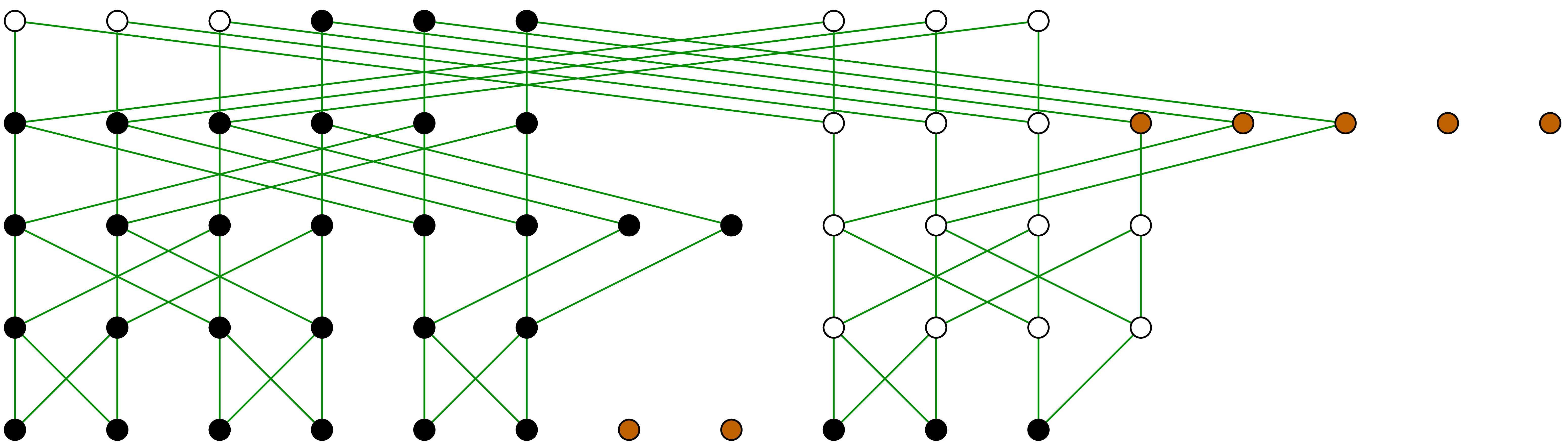
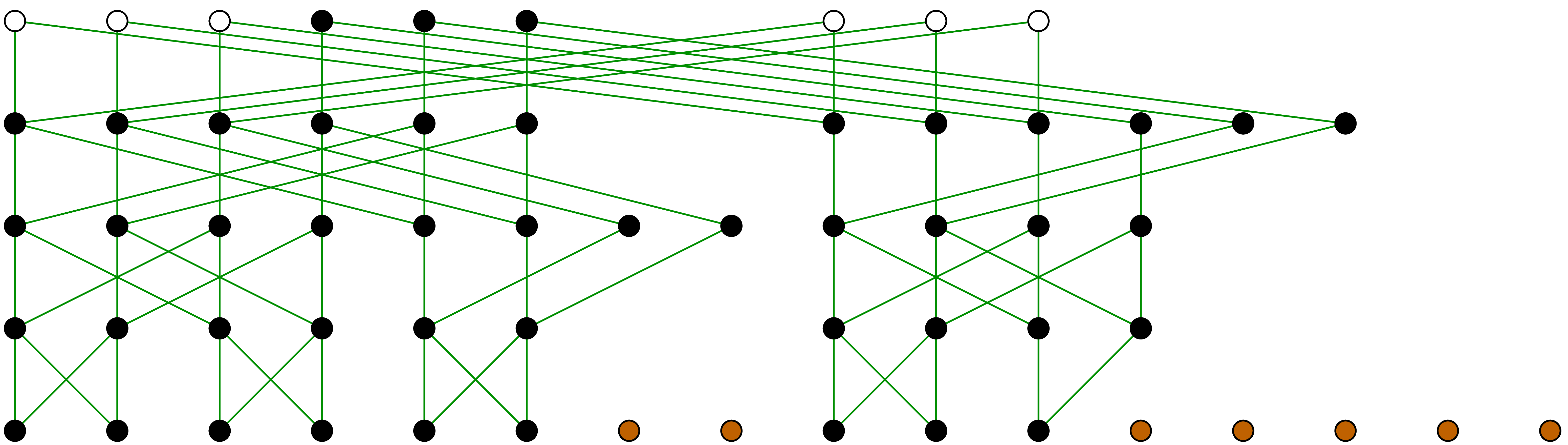
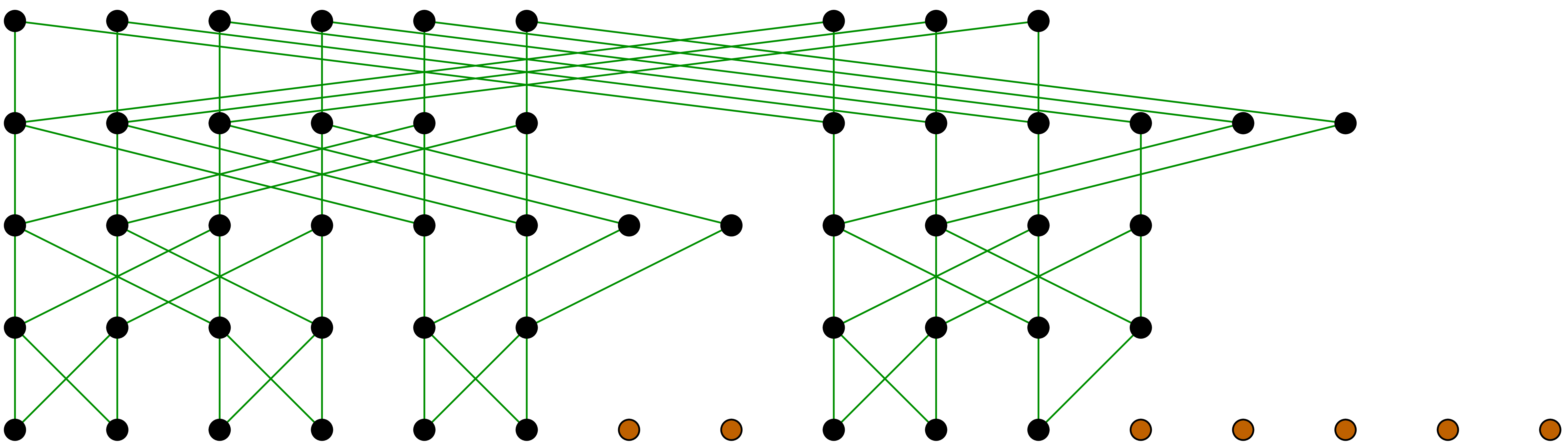
In order to compute the TFT, we simply consider the computation graph of
a complete FFT and throw out all computations which do not contribute to
the result  (see figures 2, 3
and 4). If the set is
“sufficiently connected”, then the cost of the computation
of is
(see figures 2, 3
and 4). If the set is
“sufficiently connected”, then the cost of the computation
of is  .
For instance, for
.
For instance, for  , we have
proved [vdH04]:
, we have
proved [vdH04]:
6.
Inverting the Truncated Fourier Transform
In order to use the TFT for the multiplication of numbers,
polynomials or power series, we also need an algorithm to compute the
inverse transform. In this section, we give such an algorithm in the
case when  and when is an
initial segment for the (partial) “bit ordering
and when is an
initial segment for the (partial) “bit ordering  ” on :
given numbers
” on :
given numbers  and
and  (with
(with
 ), we set
  if
if  for all .
We recall that an initial segment of is a set
with
for all .
We recall that an initial segment of is a set
with  .
.
The inverse TFT is based on the key observation that the cross relation
can also be applied to compute “one diagonal from the other
diagonal”. More precisely, given a relation
 |
(5) |
where  for some ,
we may clearly compute
for some ,
we may clearly compute  as a function of
  and vice versa
 |
(6) |
but we also have
Moreover, these relations only involve shifting (multiplication and
division by ), additions,
subtractions and multiplications by roots of unity.
In order to state our in-place algorithm for computing the inverse TFT,
we will need some more notations. At the very start, we have  and
and  on input, where
  is the complement of in
  and is the zero function. Roughly
speaking, the algorithm will replace by its
inverse TFT
and is the zero function. Roughly
speaking, the algorithm will replace by its
inverse TFT  and by its
direct TFT
and by its
direct TFT  . In the actual
algorithm, the array will be stored in a special
way (see the next section) and only a part of the computation of will really be carried out.
. In the actual
algorithm, the array will be stored in a special
way (see the next section) and only a part of the computation of will really be carried out.
Our algorithm proceeds by recursion. In the recursive step,  is replaced by a subset of of the
form
is replaced by a subset of of the
form  , where
is the current step and
, where
is the current step and  . The
sets and will again be
subsets of with
. The
sets and will again be
subsets of with  ,
and
,
and  is recursively assumed to be an initial
segment for the bit ordering. Given a subset
is recursively assumed to be an initial
segment for the bit ordering. Given a subset  of
, we will denote
of
, we will denote  and
and  , where

Similarly, given  , we will
denote by
, we will
denote by  and
and  the
restrictions of
the
restrictions of  to
to  resp.
resp.  . We now
have the following recursive in-place algorithm for computing the
inverse TFT (see figure 5 for an illustration of the
different steps).
. We now
have the following recursive in-place algorithm for computing the
inverse TFT (see figure 5 for an illustration of the
different steps).
Algorithm 
If  or
or  then return
If  then apply the partial inverse FFT on
  and return
Applying the algorithm for with  , we have
Remark 3. Even though it
seems that the linear transformation  has a
non-zero determinant for any
has a
non-zero determinant for any  ,
an algorithm of the above kind does not always work. The simplest
example when our method fails is for
,
an algorithm of the above kind does not always work. The simplest
example when our method fails is for  and
and  . Nevertheless, the condition that
is an initial segment for the bit ordering on
. Nevertheless, the condition that
is an initial segment for the bit ordering on
 is not a necessary condition. For instance, a
slight modification of the algorithm also works for final segments and
certain more general sets like
is not a necessary condition. For instance, a
slight modification of the algorithm also works for final segments and
certain more general sets like  for
for  . We will observe in the next section that the
bit ordering condition on is naturally satisfied
when we take multivariate TFTs on initial segments of
. We will observe in the next section that the
bit ordering condition on is naturally satisfied
when we take multivariate TFTs on initial segments of  .
.
7.The multivariate TFT
Let  and let
  be a
primitive -th root of unity
for each . Given subsets
be a
primitive -th root of unity
for each . Given subsets  of
of  and a mapping
  , the multivariate TFT of
is a mapping
, the multivariate TFT of
is a mapping  defined by

See figure 6 for an example with in
dimension  . The multivariate
TFT and its inverse are computed in a similar way as in the univariate
case, using one of the encodings from see section 3 of
tuples in by integers in
. The multivariate
TFT and its inverse are computed in a similar way as in the univariate
case, using one of the encodings from see section 3 of
tuples in by integers in  and using the corresponding FFT-profile determined by
instead of
and using the corresponding FFT-profile determined by
instead of  .
.
We generalize the bit-ordering on sets of the
form  to sets of indices
by
to sets of indices
by

If  is one of the encodings
  or
or  from section
  ,
then it can be checked that
,
then it can be checked that

If is an initial segment for the bit ordering,
this ensures that the inverse TFT also generalizes to the multivariate
case.
 |
|
Figure 6. Illustration of a
TFT in two variables ( ). ).
|
From the complexity analysis point of view, two special cases are
particularly interesting. The first block case is when  with
with  for all . Then using the lexicographical encoding, the
multivariate TFT can be seen as a succession of
univariate TFTs whose coefficients are mappings
for all . Then using the lexicographical encoding, the
multivariate TFT can be seen as a succession of
univariate TFTs whose coefficients are mappings  , with

Setting  ,
,  and
and  , theorems 1
and 2 therefore generalize to:
, theorems 1
and 2 therefore generalize to:
Remark 5. The power series
analogue of the block case, i.e. the problem of
multiplication in the ring  is also an
interesting. The easiest instance of this problem is when
is also an
interesting. The easiest instance of this problem is when  for some
  . In
that case, we may introduce a new variable
. In
that case, we may introduce a new variable  and
compute in
and
compute in  instead of
  , where
  is the smallest
power of two with
is the smallest
power of two with  . This
gives rise to yet another FFT-profile of the form
. This
gives rise to yet another FFT-profile of the form  and a complexity in
  . The
trick generalizes to the case when the
. The
trick generalizes to the case when the  are all
powers of two, but the general case seems to require non-binary FFT
steps.
are all
powers of two, but the general case seems to require non-binary FFT
steps.
The other important simplicial case is when  and
and  for some fixed
  with
with
 (and more generally, one may consider weighted
degrees). In this case, we choose the simultaneous encoding for the
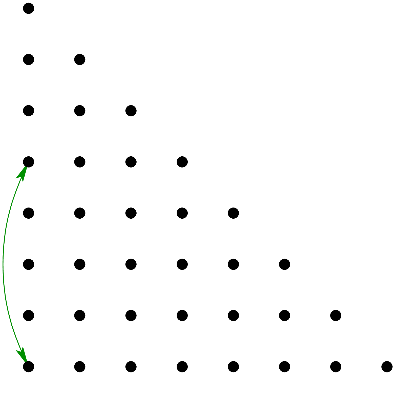
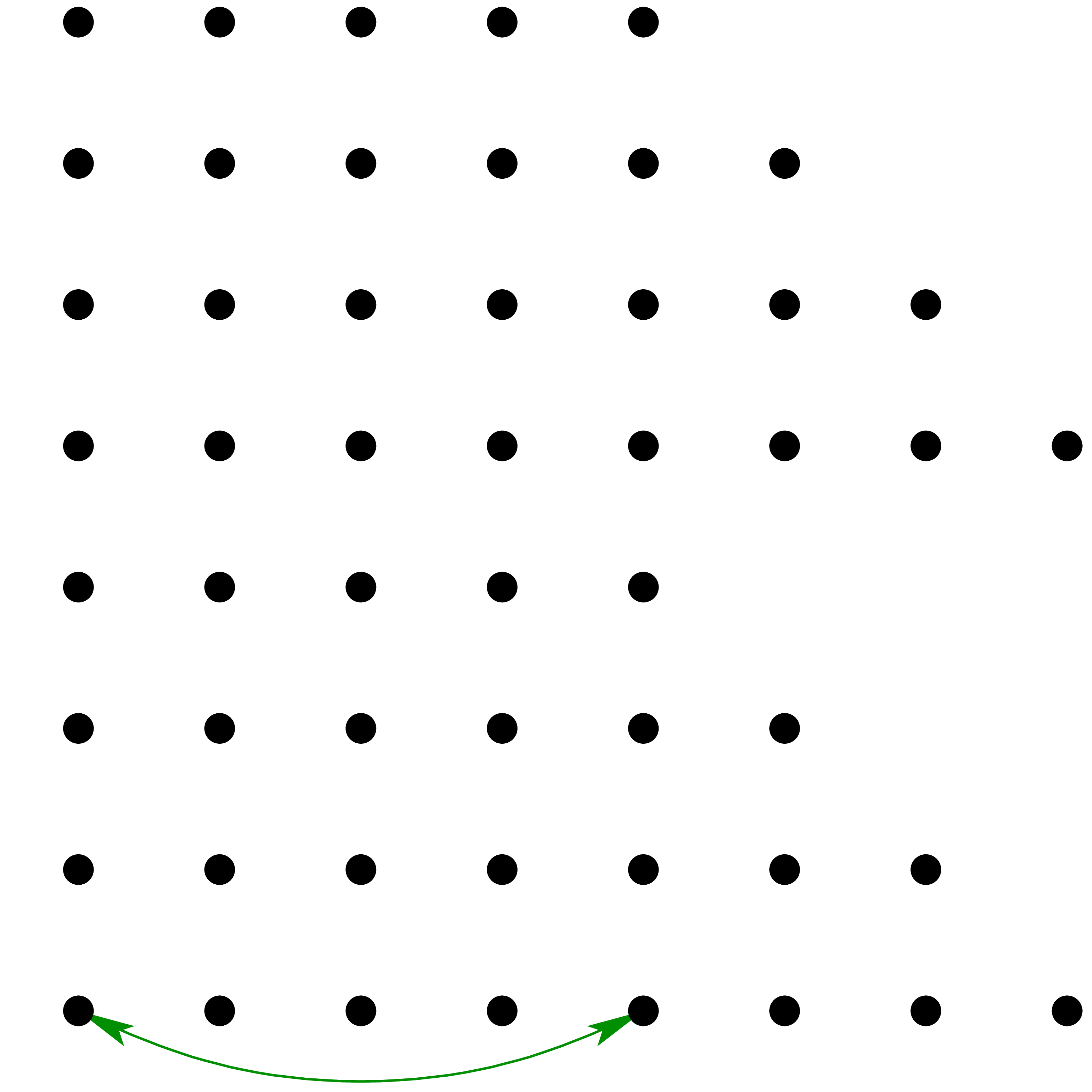
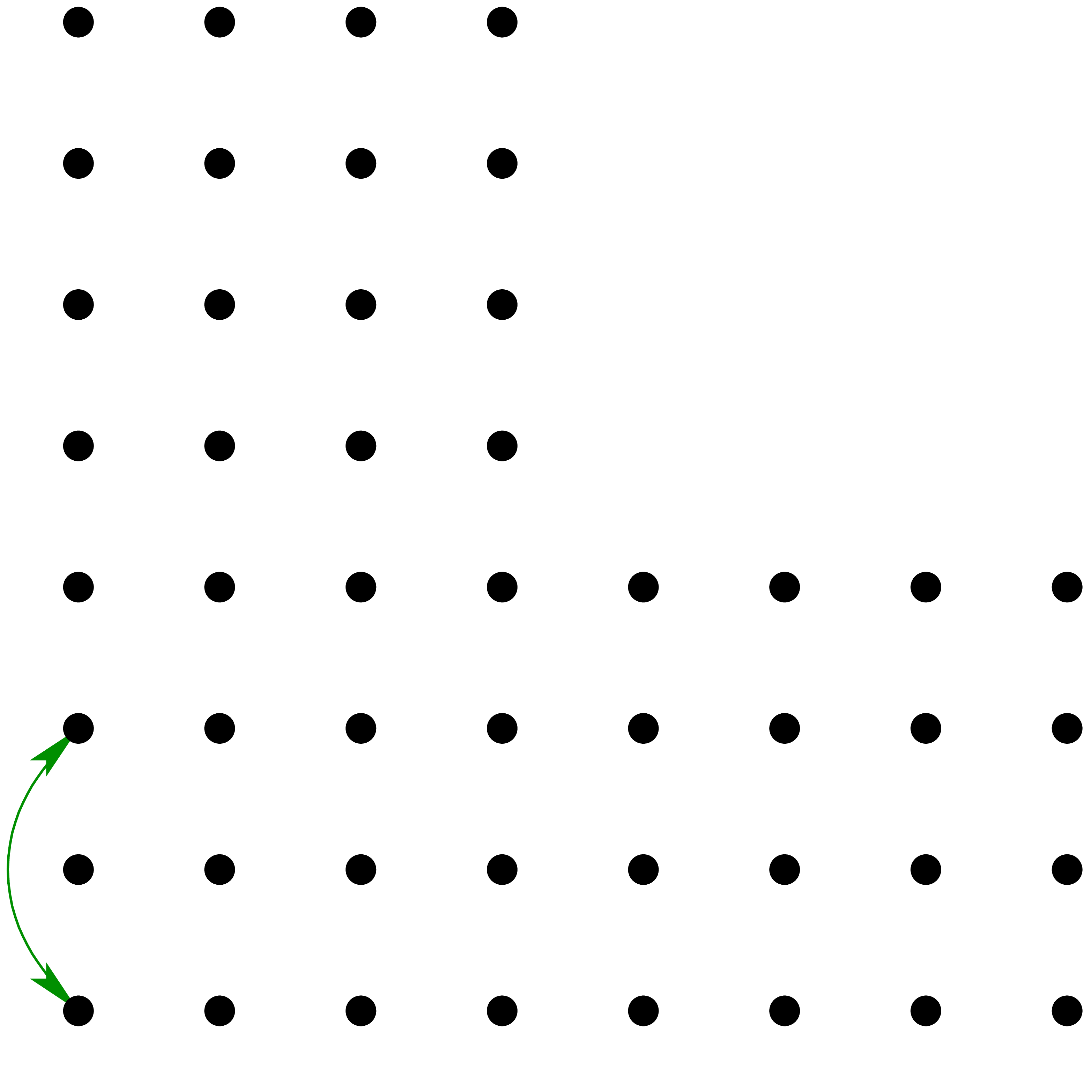
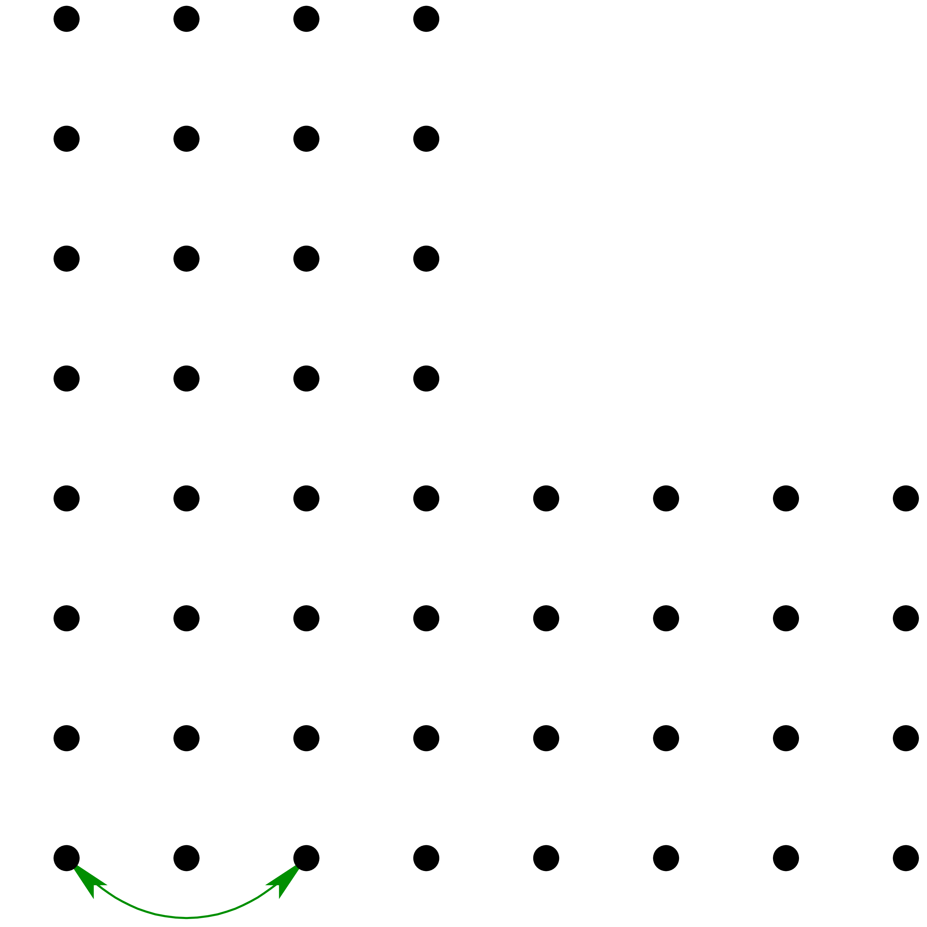
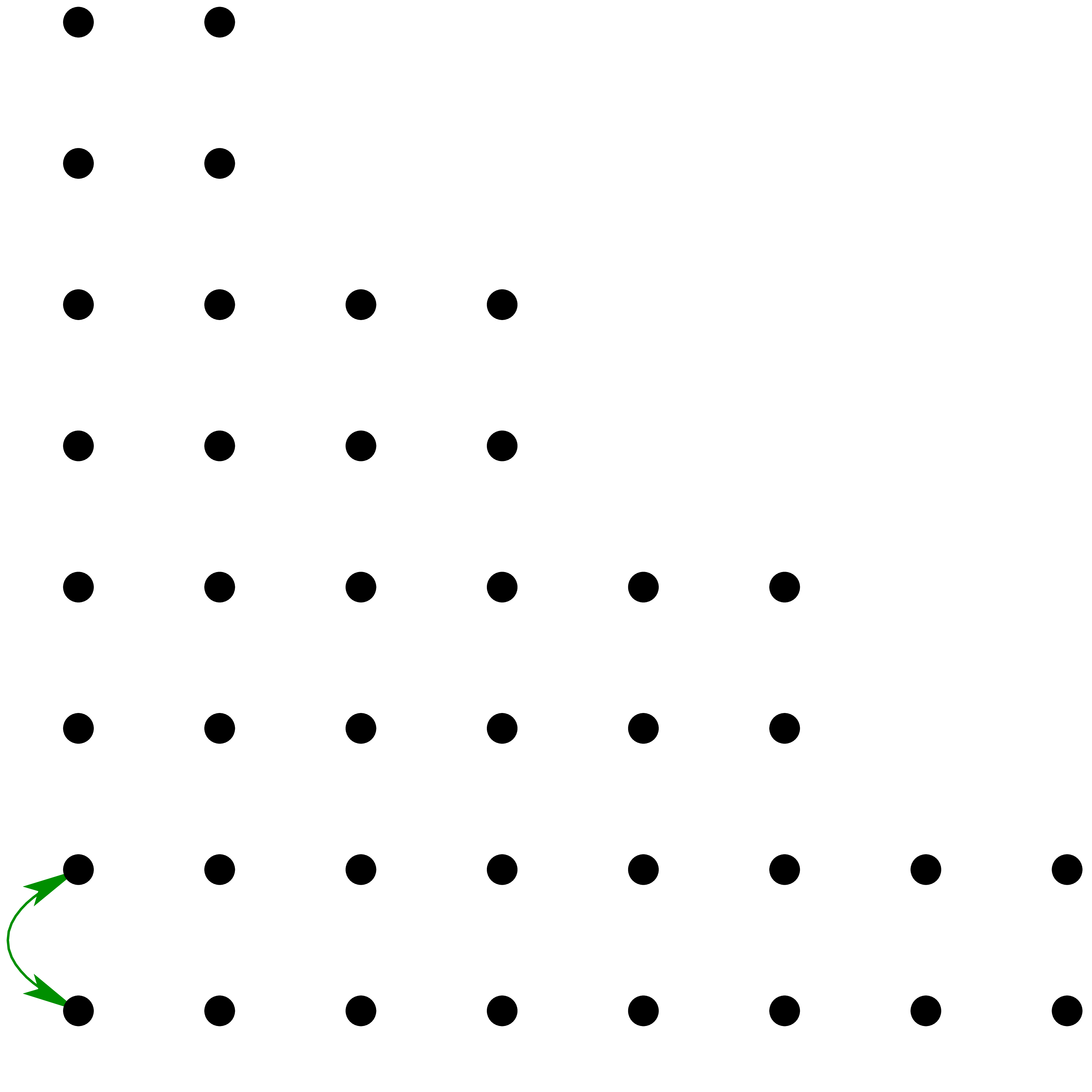
multivariate TFT (see figure 7 for an example). Now the
size of is
(and more generally, one may consider weighted
degrees). In this case, we choose the simultaneous encoding for the
multivariate TFT (see figure 7 for an example). Now the
size of is  .
At stages
.
At stages  , we notice that
the number of “active nodes” for the TFT is bounded by
, we notice that
the number of “active nodes” for the TFT is bounded by  . When
  , we have

which proves:
Remark 7. The complexity
analysis of the simplicial case in [vdH04, Section 5]
contained a mistake. Indeed, for the multivariate TFT described there,
the computed transformed coefficient  does not
depend on
does not
depend on  , which is
incorrect.
, which is
incorrect.
Remark 8. Theorem 6
may be used to multiply formal power series in a similar way as in [vdH04]. This multiplication algorithm requires an additional
logarithmic overhead. Contrary to what was stated in [vdH04],
we again need the assumption that .
|
|
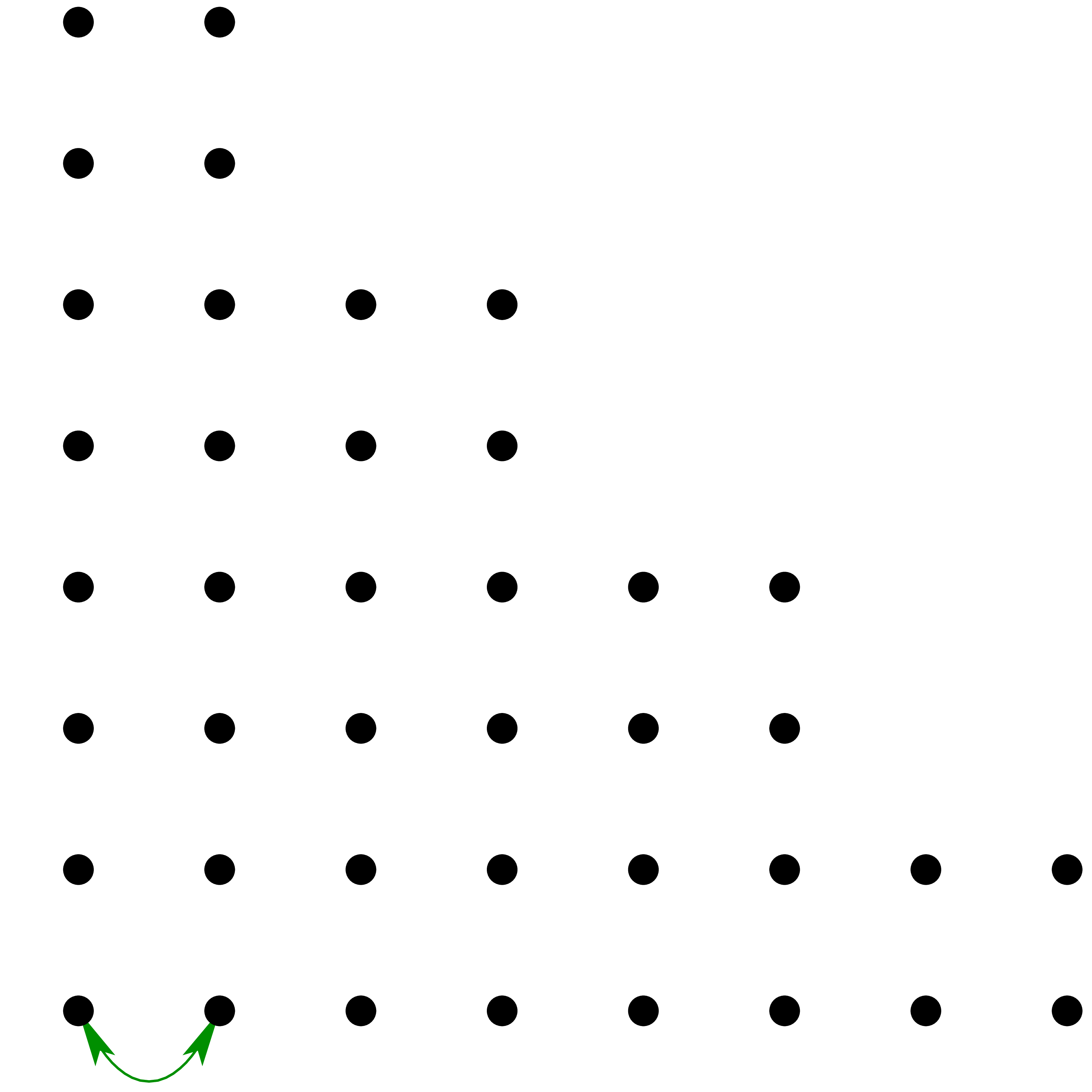
Figure 7. Illustration of the
different stages of a bivariate simplicial TFT for  . The black dots correspond to the
active nodes at each stage. The arrows indicate two nodes which
will be crossed between the current and the next stage. . The black dots correspond to the
active nodes at each stage. The arrows indicate two nodes which
will be crossed between the current and the next stage.
|
8.Implementing the TFT
In order to implement the TFT and its inverse, one first has to decide
how to represent the sets and , and mappings .
A convenient approach is to represent ,
and (for the direct TFT)
or ,
and (for the inverse TFT) by a single binary
“TFT-tree”. Such a binary tree corresponds to what happens
on a subset  of the form
  with
with  . The binary tree is of
one of the following forms:
. The binary tree is of
one of the following forms:
-
Leafs
-
When the tree is reduced to a leaf, then it explicitly contains a
map  , which is
represented by an array of length
, which is
represented by an array of length  in
memory. By convention, if is reduced to a
null-pointer, then represents the zero
map. Moreover, the node contains a flag in order to indicate
whether
in
memory. By convention, if is reduced to a
null-pointer, then represents the zero
map. Moreover, the node contains a flag in order to indicate
whether  or
or  (for
leafs, it is assumed that we either have
or
(for
leafs, it is assumed that we either have
or  and similarly for ).
-
Binary nodes
-
When the tree consists of a binary node with subtrees  and
and  ,
then encodes what happens on the interval
,
then encodes what happens on the interval
 , whereas encodes what happens on the interval
  . For convenience, the tree still
contains a flag to indicate whether
. For convenience, the tree still
contains a flag to indicate whether  or
or
 .
.
Notice that the bounds of the interval  need not
to be explicitly present in the representation of the tree; when needed,
they can be passed as parameters for recursive functions on the trees.
need not
to be explicitly present in the representation of the tree; when needed,
they can be passed as parameters for recursive functions on the trees.
Only the direct TFT has currently been implemented in Mmxlib.
This implementation roughly follows the above ideas and can be used in
combination with arbitrary FFT-profiles. However, the basic arithmetic
with “TFT-trees” has not been very well optimized yet.
In tables 1–4, we have given a few
benchmarks on a 2.4GHz AMD architecture with 512Mb of memory. We use
 as our coefficient ring and we tested the
simplicial multivariate TFT for total degree and
dimension . Our table both
shows the size of the input
as our coefficient ring and we tested the
simplicial multivariate TFT for total degree and
dimension . Our table both
shows the size of the input  ,
the real and average running times
,
the real and average running times  and
and  , the theoretical number of
crossings to be computed
, the theoretical number of
crossings to be computed  ,
its average
,
its average  and the ratio
  . The number
  correspond to
the running time divided by the running time of the univariate TFT for
the same input size. The tables both show the most favourable cases when
is a power of two and the worst cases when is a power of two plus one.
correspond to
the running time divided by the running time of the univariate TFT for
the same input size. The tables both show the most favourable cases when
is a power of two and the worst cases when is a power of two plus one.
9.Improving the implementation of the TFT
A few conclusions can be drawn from tables 1–4.
First of all, in the univariate case, the TFT behaves more or less as
theoretically predicted. The non-trivial ratios  in higher dimensions indicate that the set is
quite disconnected. Hence, optimizations in the implementation of
TFT-trees may cause non-trivial gains. The differences between the
running times for the best and worse cases in higher dimensions show
that the multivariate TFT is still quite sensible to the jump phenomenon
(even though less than a full FFT). Finally, in the best case, the ratio
be comes reasonably small. Indeed, should theoretically tend to
in higher dimensions indicate that the set is
quite disconnected. Hence, optimizations in the implementation of
TFT-trees may cause non-trivial gains. The differences between the
running times for the best and worse cases in higher dimensions show
that the multivariate TFT is still quite sensible to the jump phenomenon
(even though less than a full FFT). Finally, in the best case, the ratio
be comes reasonably small. Indeed, should theoretically tend to  and
should be bounded by ! in
order to gain something w.r.t. a full FFT. However, can become quite large in the worse case. The various
observations suggest the following future improvements.
and
should be bounded by ! in
order to gain something w.r.t. a full FFT. However, can become quite large in the worse case. The various
observations suggest the following future improvements.
Avoiding expression swell
In the case of simplicial TFTs, the number of active nodes swells
quite dramatically at the first stages of the TFT (the size may
roughly be multiplied by a factor
).
In this special case, it may therefore be good to compress the first
steps into a single step. Moreover, one
benefits from the fact that this compression can be done in a
particularly efficient way. Indeed, let

be the
transform of

after
steps. We have

for all  and
and

for each  . It can be hoped
that this acceleration approximately reduces the current running times
for the worst case to the current running times for the best case. For
high dimensions, it may be useful to apply the trick a second time for
the next stages
. It can be hoped
that this acceleration approximately reduces the current running times
for the worst case to the current running times for the best case. For
high dimensions, it may be useful to apply the trick a second time for
the next stages  ;
however, the corresponding formulas become more complicated. We hope
that further study will enable the replacement of the condition in theorem 6 by a better condition, like
;
however, the corresponding formulas become more complicated. We hope
that further study will enable the replacement of the condition in theorem 6 by a better condition, like
 .
.
Avoiding small leafs
At the other back-end, the overhead in the manipulation of TFT-trees
may be reduced by allowing only for leafs whose corresponding arrays
have a minimal size of
,
 ,
,  ,
, or more. Also, if the intersection of
with the interval
of a TFT-tree
has a high density (say
 ),
),
then we may replace the TFT-tree by a leaf.
Reducing the jump phenomenon
When the TFT is used for polynomial or power series multiplication,
and
is slightly above a power of two
, then classical techniques may
be used for reducing the jump phenomenon. For instance, the
polynomials
and
may be
decomposed

and
 ,
,
where

is the part of total degree
 ,
, 
and similarly for
. Then

is computed using the TFT at order
and the
remainder

by a more naive method.
10.The TFT for real coefficients
Assume now that is a ring such that  has many -th
roots of unity. Typically, this is the case when
is the “field” of floating point numbers. A disadvantage of
the standard FFT or TFT in this context is that the size of the input is
doubled in order to represent numbers in .
This doubling of the size actually corresponds to the fact that the FFT
or TFT contains redundant information in this case. Indeed, given
has many -th
roots of unity. Typically, this is the case when
is the “field” of floating point numbers. A disadvantage of
the standard FFT or TFT in this context is that the size of the input is
doubled in order to represent numbers in .
This doubling of the size actually corresponds to the fact that the FFT
or TFT contains redundant information in this case. Indeed, given  with , we
have
with , we
have  for any -th
root of unity . This suggests
to evaluate either in or
for any -th
root of unity . This suggests
to evaluate either in or
 .
.
With the notations from section 5, let  be an initial segment for the bit ordering .
As our target set , we take
be an initial segment for the bit ordering .
As our target set , we take

The “real TFT” now consists of applying the usual TFT with
source and target .
It can be checked that crossings of “real nodes” introduce
“complex nodes” precisely then when one of the two nodes
disappears at the next stage (see figure 8). It can also be
checked that the inverse TFT naturally adapts so as to compute the
inverse real TFT. For “sufficiently connected” sets , like , the real TFT is asymptotically twice as fast as
the complex TFT.
 |
|
Figure 8. Schematic representation
of a real FFT. The white nodes correspond to real numbers and
the black nodes to complex numbers.
|
Bibliography
-
[CK91]
-
D.G. Cantor and E. Kaltofen. On fast multiplication
of polynomials over arbitrary algebras. Acta
Informatica, 28:693–701, 1991.
-
[CT65]
-
J.W. Cooley and J.W. Tukey. An algorithm for the
machine calculation of complex Fourier series. Math.
Computat., 19:297–301, 1965.
-
[SS71]
-
A. Schönhage and V. Strassen. Schnelle
Multiplikation grosser Zahlen. Computing
7, 7:281–292, 1971.
-
[vdH02]
-
J. van der Hoeven. Relax, but don't be too lazy.
JSC, 34:479–542, 2002.
-
[vdH04]
-
J. van der Hoeven. The truncated Fourier transform
and applications. In J. Gutierrez, editor, Proc.
ISSAC 2004, pages 290–296, Univ. of Cantabria,
Santander, Spain, July 4–7 2004.
-
[vdHea05]
-
J. van der Hoeven et al. Mmxlib: the standard library
for Mathemagix, 2002–2005.
ftp://ftp.mathemagix.org/pub/mathemagix/targz.
 .
. ,
, and the lower row
 .
. and let
  be a primitive
  -th
-th .
. -tuple
 w.r.t.
 can be computed using at most
  additions (or subtractions) and
  multiplications with powers of
 .
.
 .
.
 .
.


 ,
, with
with  using (
 ,
, with
with 
 ,
, using (
 .
. (the
black dots) during the different computations at stage
(the
black dots) during the different computations at stage  .
. shifted additions (or subtractions) and
  multiplications with powers of the
  .
. shifted additions (or subtractions) and multiplications with powers of
 .
.


 in μs
in μs
 .
.